Speeding Up Physical Failure Analysis (PFA)

The cost of an IC depends on many factors like: NRE, masks, fabrication, testing, packaging. Product engineers are tasked with testing each part and understanding what exactly is limiting the yields. Every company has a methodology for Physical Failure Analysis (PFA), and the challenge is to make this process as quick as possible, because time is money especially when using testers that can cost millions of dollars.

Volume scan diagnostics is a popular method for creating defect paretos and plotting yield, and the larger the sampling size the better the accuracy. There are many challenges for product engineers these days:

• Larger design sizes slow down testing
• New process nodes have new failure mechanisms
• Cell-aware diagnosis takes more time
• Compute resources are growing

Let’s take a closer look at what happens during volume scan diagnosis; a design netlist is read into a simulator along with scan patterns and the log from a failing chip. To handle multiple fail logs quickly the diagnosis is simulated in parallel across a grid of computers.

With large designs there can be practical computational limits to scan diagnosis, so let’s assume that your design takes 100GB of RAM and requires an hour for each diagnosis. If your compute grid has 11 machines as shown below:

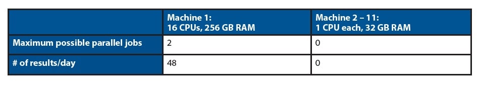
Only Machine 1 has enough RAM to fit the design and with 2 parallel jobs it will diagnose only 48 results per day. Machines 2-11 don’t have enough RAM to fit the design, so they remain idle.

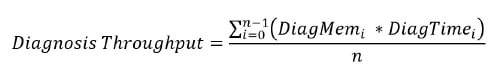
The actual diagnosis throughput can be described as an equation that depends on how much diagnosis memory and diagnostic time is required.

To shorten the diagnosis throughput requires that we somehow reduce the memory and time requirements, and it turns out that a technique called Dynamic Partitioning as used in the Tessent Diagnosis tool from Mentor does this.

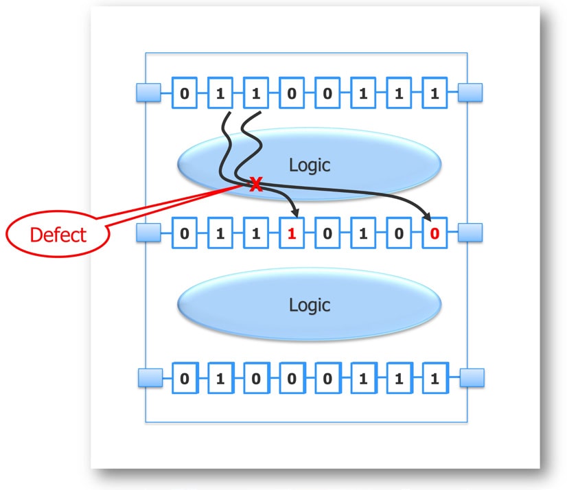
In the following figure we see a design fragment with three scan chains, and a defect is found in the top logic cloud which then causes two scan bits to fail in the second scan chain shown as red logic values. Using dynamic partitioning only this design fragment needs to be simulated by Tessent Diagnosis, thus requiring much less RAM than a full netlist.

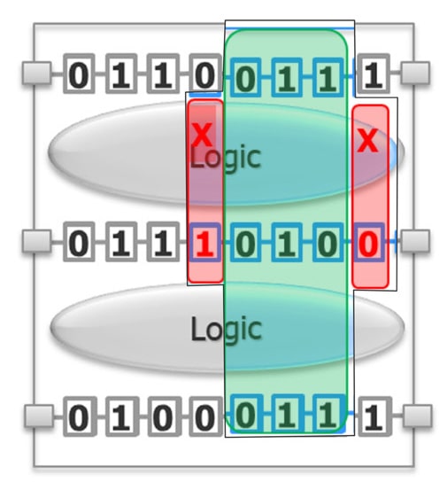
Here’s the smaller partition that needs to be simulated:

With Tessent Diagnosis Server all of the dynamic partitioning is automated and it works with your compute grid setup, like LSF, so that run times are minimized.

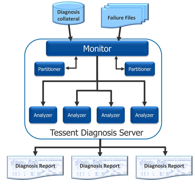
You can even choose the number of partitioners and analyzers to be used on your grid, where the partitioners automatically create dynamic partitions for diagnosis and analyzers do the diagnosis on the smaller partitions.

Let’s go back to the first test case and this time apply dynamic partitioning:

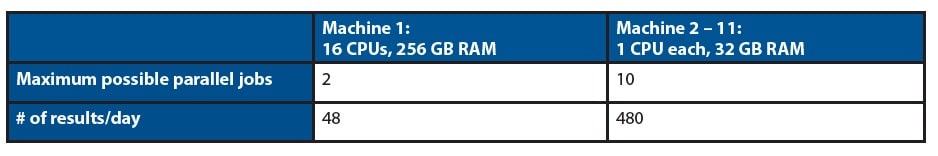
With dynamic partitioning the diagnosis throughput jumps from 48 results/day up to 528 results/day because all 11 machines can be utilized in parallel. Two test cases from actual designs show throughput improvements between 11X and 16X faster by using dynamic partitioning:

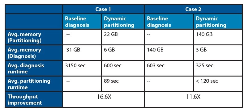
When using dynamic partitioning there’s no change in the quality of the scan diagnosis result, you just get back results much quicker from your compute grid using less RAM.

Summary

Divide and conquer is a proven approach to simplifying EDA problems and for product engineers doing PFA there’s some welcome relief in improving throughput based on dynamic partitioning technology. The old adage, “Work smarter, not harder”, applies again in this case because you can now use your compute grid more efficiently to shorten volume scan diagnosis.

Read the complete 6 page White Paper online, after a short registration process.

Related Blogs

• Can a hierarchical Test flow be used on a flat design?
• Automotive Market Pushing Test Tool Capabilities
• Hierarchical RTL Based ATPG for an ARM A75 Based SOC