AI Inference at the Edge – Architecture and Design

In the old days, product architects would throw a functional block diagram “over the wall” to the design team, who would plan the physical implementation, analyze the timing of estimated critical paths, and forecast the signal switching activity on representative benchmarks.  A common reply back to the architects was, “We’ve evaluated the preliminary results against the power, performance, and cost targets – pick two.”  Today, this traditional “silo-based” division of tasks is insufficient.  A close collaboration between architecture and design addressing all facets of product development is required.  This is perhaps best exemplified by AI inference engines at the edge, where there is a huge demand for analysis of image data, specifically object recognition and object classification (typically in a dense visual field).

The requirements for object classification at the edge differ from a more general product application.  Raw performance data – e.g., maximal operations per section (TOPS) – is less meaningful.  Designers seek to optimize the inference engine frames per second (fps), frames per watt (fpW), and frames per dollar (fp$).  Correspondingly, architects must address the convolutional neural network (CNN) topologies that achieve high classification accuracy, while meeting the fps, fpW, and fp$ product goals.  This activity is further complicated by the rapidly evolving results of CNN research – the architecture must also be sufficiently extendible to support advances in CNN technology.

Background

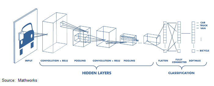
AI inference for analysis of image data consists of two primary steps – please refer to the figure below.

Feature extraction commonly utilizes a (three-dimensional) CNN, supporting the two dimensions of the pixel image plus the (RGB) color intensity.  A convolutional filter is applied to strides of pixels in the image.  The filter matrix is a set of learned weights.  The size of the filter coefficient array is larger than the stride to incorporate data from surrounding pixels, to identify distinct feature characteristics.  (The perimeter of the image is “padded” with data values, for the filter calculation at edge pixels.)  The simplest example would use a 3×3 filter with a stride of 1 pixel.  Multiple convolution filters are commonly applied (with different feature extraction properties), resulting in multiple feature maps for the image, to be combined as the output of the convolution layer.  This output is then provided to a non-linear function, such as Rectified Linear Unit (ReLU), sigmoid, tanh, softmax, etc.

The dimensionality of the data for subsequent layers in the neural network is reduced by pooling – various approaches are used to select the stride and mathematical algorithm to reduce the dataset to a smaller dimension.

Feature extraction is followed by object classification.  The data from the CNN layers is flattened and input to a conventional, fully-connected neural network, whose output identifies the presence and location of the objects in the image, from the set of predefined classes used during training.

Training of a complex CNN is similar to that of a conventional neural network.  A set of images with identified object classes is provided to the network.  The architect selects the number and size of filters and the stride for each CNN layer.  Optimization algorithms work backward from the final classification results on the image set, to update the CNN filter values.

Note that the image set used for training is often quite complex.  (For example, check out the Microsoft COCO, PASCAL VOC, and Google Open Images datasets.)  The number of object classes is large.  Objects may be scaled in unusual aspect ratios.  Objects may be partially obscured or truncated.  Objects may be present in varied viewpoints and diverse lighting conditions.  Object classification research strives to achieve greater accuracy on these training sets.

Early CNN approaches applied “sliding windows” across the image for analysis.  Iterations of the algorithm would adaptively size the windows to isolate objects in bounding boxes for classification.  Although high in accuracy, the computational effort of this method is extremely high and the throughput is low – not suitable for inference at the edge.  The main thrust for image analysis requiring real-time fps throughput is to use full-image, one-step CNN networks, as was depicted in the figure above.  A single convolutional network simultaneously predicts multiple bounding boxes and object class probabilities for those boxes.  Higher resolution images are needed to approach the accuracy of region-based classifiers.  (Note that a higher resolution image also improves extraction for small objects.)

Edge Inference Architecture and Design

I recently had the opportunity to chat with the team at Flex Logix, who recently announced a product for AI inference at the edge, InferX X1.  Geoff Tate, Flex Logix CEO, shared his insights into how the architecture and design teams collaborated on achieving the product goals.

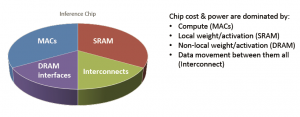
“We were focused on the optimizing inferences per watt and inferences per dollar for high-density images, such as one to four megapixels.”, Geoff said.  “Inference engine chip cost is strongly dependent on the amount of local SRAM, to store weight coefficients and intermediate layer results – that SRAM capacity is balanced against the power associated with transferring weights and layer data to/from external DRAM.  For power optimization, the goal is to maximize MAC utilization for the neural network – the remaining data movement is overhead.”

For a depiction of the memory requirements associated with different CNN’s and image sizes, Geoff shared the chart below.  The graph shows the maximum memory to store weights and data for network layers n and n+1.

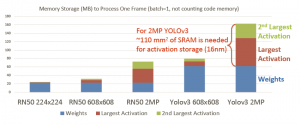
The figure highlights the amount of die area required to integrate sufficient local SRAM for the n/n+1 activation layer evaluation — e.g., 160MB for YOLOv3 and a 2MP image, with the largest activation layer storage of ~67MB.  This memory requirement would not be feasible for a low-cost edge inference solution.

Geoff continued, “We evaluated many design tradeoffs with regards to the storage architecture, such as the amount of local SRAM (improved fps, higher cost) versus the requisite external LPDDR4 capacity and bandwidth (reduced fps, higher power).  We evaluated the MAC architecture appropriate for edge inference – an “ASIC-like’ MAC implementation is needed at the edge, rather than a general-purpose GPU/NPU.  For edge inference on complex CNN’s, the time to reconfigure the hardware is also critical.  Throughout these optimizations, the focus was on supporting advanced one-step algorithms with high pixel count images.”

The final InferX X1 architecture and physical design implementation selected by the Flex Logix team is illustrated in the figure below.

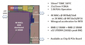
The on-chip SRAM is present in two hierarchies:  (1) distributed locally with clusters of the MAC’s (providing 8×8 or 16×8 computation) to store current weights and layer calculations, and (2) outside the MAC array for future weights.

The MAC’s are clustered into groups of 64.  “The design builds upon the expertise in MAC implementations from our embedded FPGA IP development.”, Geoff indicated.  “However, edge inference is a different calculation, with deterministic data movement patterns known at compile time.  The granularity of general eFPGA support is not required, enabling the architecture to integrate the MAC’s into clusters with distributed SRAM.  Also, with this architecture, the internal MAC array can be reconfigured in less than 2 microseconds.”

Multiple smaller layers can be “fused” into the MAC array for pipelined evaluation, reducing the external DRAM bandwidth – the figure below illustrates two layers in the array (with a ReLU function after the convolution).  Similarly, the external DRAM data is loaded into the chip for the next layer in the background, while the current layer is evaluated.

Geoff provided benchmark data for the InferX X1 design, and shared a screen shot from the InferX X1 compiler (TensorFlowLite), providing detailed performance calculations – see the figure below.

“The compiler and performance modeling tools are available now.”, Geoff indicated.  “Customer samples of InferX X1 and our evaluation board will be available late Q1’2020.”

I learned a lot about inference requirements at the edge from my discussion with Geoff.  There’s a plethora of CNN benchmark data available, but edge inference requires laser focus by architecture and design teams on fps, fpW, fp$, and accuracy goals, for one-step algorithms with high pixel images.  As CNN research continues, designs must also be extendible to accommodate new approaches.  The Flex Logix InferX X1 architecture and design teams are addressing those goals.

For more info on InferX X1, please refer to the following link.

-chipguy