SemiWiki – Page 322 – The Open Forum for Semiconductor Professionals

RVN! 26 Banner revised (800 x 100 px) (600 x 100 px)

March 10, 2021March 16, 2022

Cadence Underlines Verification Throughput at DVCon

Cadence Underlines Verification Throughput at DVCon
by Bernard Murphy on 03-10-2021 at 6:00 am
Categories: Cadence, EDA, Events

Paul Cunningham, CVP and GM of the System Verification Group at Cadence gave the afternoon Keynote on Tuesday at DVCon and doubled down on his verification-throughput message. At the end of the day, what matters most to us in verification is the number of bugs found and fixed per dollar per day. You can’t really argue with that message. This is the ultimate metric for semiconductor product verification. Cycles per second, debug features, this engine versus that engine—these are ultimately mechanisms for delivering that outcome.

Throughput starts with best in class engines

That’s not to say that cycles per second and so on are unimportant. Paul has a very grounded engineering viewpoint. The horsepower underneath this throughput needs to be the best of the best in each instance. But, on top of that, what Paul (and Anirudh) call logistics—the most effective use of these resources to meet that ultimate goal—have become just as important. This view draws on an analogy with package delivery in our increasingly online world. Planes are used for long-distance transportation, long-haul trucks for plane-to-warehouse transportation and vans for last-mile delivery/pickup. Each mode has strengths and weaknesses: Speed versus setup time versus reach. Logistics is about combining these effectively to maximize throughput.

The same applies in verification. Simulation is the last-mile equivalent; emulation is the long-haul truck, and FPGA prototyping is the fastest throughput with longest time to setup. Paul added that no analogy is perfect; in verification we also have formal, which plays an important role in this throughput story. Maybe the physical logistics people need to find a parallel to up their game!

Logistics and machine learning

But having fast planes and trucks and vans is not enough to maximize throughput. FedEx, UPS and others put huge investments into scheduling and routing traffic to meet their throughput goals. The same principle must be applied to verification, for which you need logistics management on top of the engines. Xcelium-ML provides an example which leverages machine learning (ML) to reduce regression runs while maintaining the same level of coverage. We all know that some number of regression cycles are low value because they’re simply proving over and over again that “even though this code didn’t change, we checked it anyway and it still works.” This is particularly important in randomized simulations, where many randomizations may be very low value. The trick is to know what tests you can drop without missing some subtle but fatal error. That’s where machine learning comes in.

Another area where ML can play a significant role is in formal proving and regressions. We often think of formal as hard because there are many different proof engines and methodologies. You may need several of these to find your way to a proof. Which method to use on what problem has in the past been seen a question requiring a lot of deep expertise in the domain. The Jasper team has captured a lot of that expertise through ML methods, to find the best engines and methodologies to quickly arrive at a proof. Or to navigate through an optimum chain of alternatives.

Logistics between emulation and prototyping

Better logistics is not always about ML. Cadence have optimized Palladium emulation and Protium FPGA prototyping for better logistics between the engines through a unified compile front-end, unified transactor support and unified hardware bridge support. When you want to run high-performance emulations with maximum debuggability on Palladium, you do so. And when you want to switch to even higher performance for embedded software debug, you switch to Protium. With a minimum of fuss. Run into a problem during a Protium debug? Switch back to Palladium for better debug insight. Logistics again. You can switch from truck to plane and back to truck as needs demand.

Optimizing engines for better throughput will always be a priority. Optimizing logistics for better throughput between regression runs and between engines is what will squeeze out the maximum in bugs found per dollar per day. Which is ultimately what we have to care about.

For more information, visit the Cadence verification portal HERE.

Also Read

TECHTALK: Hierarchical PI Analysis of Large Designs with Voltus Solution

Finding Large Coverage Holes. Innovation in Verification

2020 Retrospective. Innovation in Verification

March 9, 2021October 30, 2021

Hearables: From Earbuds to Life Augmentation and Beyond

Hearables: From Earbuds to Life Augmentation and Beyond
by Kalar Rajendiran on 03-09-2021 at 10:00 am
Categories: IoT, IP, Minima Processor

Hearables Market Players Source IDTechEx Research

As the months of 2020 passed by, I started noticing more and more people sporting what looked like fashionable ear accessories. I’m of course referring to True Wireless Stereo (TWS) earbuds. With the rapid increase in online meetings due to social distancing requirements, it appeared that adoption of TWS earbuds was even faster than during the prior years. It was hard to believe that just a little more than four years ago, people had pushed back when Apple dropped support for the headphone jack in favor of their branded version of wireless earbuds (marketed as AirPods). My curiosity was piqued. I wanted to learn what was in store not just for the earbuds market but for the broader product category called Hearables, under which earbuds fall into. The term Hearables was introduced in April of 2014 simultaneously by Apple in the context of their acquisition of Beats Electronics and by product designer and wireless applications specialist Nick Hunn in a blogpost about a wearable technologies internet platform. Interestingly, the initial description for hearable technology seems to have come from a company called Valencell back in 2006. Valencell described it as a wearable ear-worn multimedia platform for health monitoring, entertainment, guidance and cloud-based communications.

Following is a summary of what I learned about the Hearables market, size, projected growth, players and market trends as well as opportunities that exist for semiconductor companies to offer valuable solutions to this market.

Market Size: According to Allied Market Research, the global hearables market size was valued at $21.90 billion in 2018 and is projected to reach $93.90 billion by 2026, growing at a CAGR of 17.2% from 2019 to 2026.

There are many players not captured in the above chart, some of whom are:

Starkey, Bragi, Doppler, Miracle-Ear, Valancell, Earin AB, Eargo, AKG, Audio-Technica, Edifier, Xiaomi, Amoi, QCY, and Anker Innovations.

Market Trends: An article titled “Hear come the Hearables”, published in the IEEE Spectrum magazine is a very interesting read and provides scientific insights into the foundational elements for the next wave of devices. The author of this article is Poppy Crum, Chief Scientist at Dolby Laboratories and an adjunct professor at Stanford University. In her article, she explains that the following data can be effectively accessed through the ears.

Heart rate
Blood oxygen levels
Movement
Temperature
Eye movements
Skin resistance
Stress hormone levels
Brain electrical activity
Vagus nerve stimulation

Note: Vagus nerve is the tenth cranial nerve, extending from its origin in the brainstem through the neck and the thorax down to the abdomen. It carries extensive range of signals from the digestive system and organs to and from the brain.

The market can be expected to offer human friendly solutions that incorporate augmented reality (AR) and IoT as applicable to immerse the user and bring a level of personal experience that has not been possible before. The next wave is going to include advanced devices that fit in our ears and leverage artificial intelligence (AI), robotics and IoT, all without interfering with our usual daily activities. The devices would be capable of recognizing one’s physiological, physical and emotional status and propose/trigger actions in response to that status.

Concerns:

Adverse long-term effects on hearing ability due to daily, prolonged use
EMF radiation exposure during to daily, prolonged use

The above types of concerns are not new. Will the next wave of devices increase these health risks?

Challenges: Maximizing battery life of these devices.

Opportunities for Semiconductor Companies:

The market opportunity for Hearables devices is big and so is the opportunity for semiconductor solutions to help implement these devices. But given the highly competitive device market with so many players, there is tremendous time to market and cost pressures.

Those semiconductor companies who are able to provide cost-effective, ultra-low power solutions to enable these devices will stand to gain a large market share. The Hearables market was an early adopter of near-threshold voltage (NTV) design techniques for its promise of ultra-low power benefit. But NTV designs have historically been difficult to implement for reliable operation.

Opportunity #1: Provide easy and cost-effective way to implement NTV designs for reliable operation. One approach may be via semiconductor IP blocks and supporting software drivers. The IP should be able to adapt the chip power usage based on real time performance needs. The solution should be programmable to the minimum energy point and still be able to step up to process user input at real time speeds.

Opportunity #2: Leverage NTV technology for energy harvesting by converting motion energy into electrical energy, thereby prolonging battery life of the hearable device.

ARM capitalized on the mobile market with its low power RISC processor cores. Similarly, an entity that enables an ultra-low power solution could capitalize on the Hearables market that is projected to rapidly grow to ~$94 billion in just a few years.

March 9, 2021March 14, 2021

A Review of Clock Generation and Distribution for Off-Chip Interfacing

A Review of Clock Generation and Distribution for Off-Chip Interfacing
by Tom Dillinger on 03-09-2021 at 6:00 am
Categories: Events, Foundries, Intel Foundry

At the recent ISSCC conference, Mozhgan Mansuri from Intel gave an enlightening (extended) short course presentation on all thing related to clocking, for both wireline and wireless interface design. [1] The presentation was extremely thorough, ranging from a review of basic clocking principles to unique circuit design strategies for synthesizing and distributing clocked signals.

Personally, I found her talk to be both an excellent refresher and a source of lots of new information (for me, at least) – I thought the highlights of her talk might be of interest to SemiWiki readers. There was a plethora of topics covered – I’ll focus on the wireline-based design considerations. I would encourage you to review her ISSCC short course material, both wireline and wireless clocking features.

Wireline DataRate Trends

A graph depicting the progress in wireline “per lane datarates” is shown below, for several interface standards.

The PPA benefits of Moore’s Law is paralleled by interface datarate enhancements, doubling every ~2-3 years. Yet, as wirelines span silicon, packaging, board interconnect, connectors, and cables, silicon technology scaling alone does not account for all of the datarate enhancements. Improvements in package/PCB materials and simulation tool advances have certainly helped.

The key to this growth has been the ongoing interface circuit enhancements supporting the Tx and Rx ends of the lane. The associated clock generation (and Rx clock recovery) techniques have been at the heart of those circuit innovations as depicted below, showing both embedded clock in data and forwarded clock options.

Clock Definitions

The basic clock definitions are shown below:

clock period
(50/50) duty cycle
clock skew (static duty cycle error, the difference between the half cycle durations)
jitter between cycles (dynamic; both deterministic (e.g., due to supply voltage variations) and random (e.g., due to thermal and flicker noise in devices))

Note in the last figure above that jitter may accumulate over time, as depicted for the odd-inverter, free-running oscillator clock source.

The figure below illustrates two key measurements (and specs) for clock distribution. The first half of the figure illustrates the frequency response of a circuit to the jitter frequency content; the second illustrates the “tolerance” of the Rx clock recovery circuitry to jitter.

The figures include a typical specification “mask” over frequency. The “ideal” jitter transfer curve depicted above provides a “0 dB, no jitter amplification” target mask through a clock distribution component. The jitter tolerance mask spec enables designers to develop the Rx clock recovery circuitry, subsequently ensuring that the Tx jitter sources do not exceed the mask limits.

Clock Synthesis Circuitry

To generate high-frequency clocks on-chip, the common method is to employ one of two main circuit types – a phase-locked loop (PLL), and a delay-locked loop (DLL). Their principal function is to provide a “multiplied” clock output derived from a lower-frequency (high-quality) reference clock, as described below. Another key clock synthesis configuration is used to phase-align individual clocks tapped from an on-die oscillator, with an “injection locked oscillator” (ILO).

PLL

The PLL consists of:

a voltage-controlled oscillator – e.g., a free-running oscillator with adaptive response to an input voltage signal that modulates the oscillator loop delay (examples given shortly)
a divide-by-N counter (the multiplicative factor of the PLL)
a phase detector, that provides an output signal proportional to the leading/lagging phase difference between the reference and divided VCO clocks (example shortly)
a low-pass filter that effectively blocks short-duration signals from the phase detector from influencing the control input to the VCO

The frequency bandwidth response of the PLL defines the jitter response, a key design tradeoff. For example, a lower bandwidth will reduce the sensitivity to jitter in the reference clock input. A higher bandwidth will reduce the sensitivity to VCO jitter.

DLL

The figure above illustrates the principles underlying a (multiplying) delay-locked loop (DLL). The free-running VCO oscillator in the PLL is replaced by a delay line, whose individual delay elements are controlled by the phase-detector and low-pass filter output – in the figure, a simple inverter delay chain is shown. The jitter in the DLL clock output is “reset” by using the reference clock edge every N cycles, using the multiplexer output providing the delay chain input – see the timing diagram in the figure.

Injection Locked Oscillator

Another option for clock synthesis is the use of injection current into an oscillating system to provide output clock phase adjust control.

A high-level block diagram of the ILO is shown below. [2] There are three components of note:

an oscillator (depicted simply as an nFET and inverting amplifier)
a tuned tank circuit
the injection current source

Recall the physics experiment where multiple metronomes of (nominally) the same time period are loosely-coupled – over time, they will synchronize (YouTube video link).

An injection current of frequency f will similarly synchronize the output voltage of the combined system to this frequency. However, due to the relative impedances of the three components, there will be a resulting phase shift between the system output voltage and the constituent currents I_tank, I_osc, and I_inj, as depicted below.

In short, Vout = (Z_tank * I_tank), where I_tank = (I_osc + I_inj). These are complex quantities with both magnitude and phase. The key feature of the ILO is that the magnitude of the injected current adjusts the phase of the output voltage.

The ILO is thus an ideal method to align (or “rotate”) the phase of a clock output, relative to a reference – the phase difference detector increases/decreases the magnitude of the injected current accordingly.

Consider the case where it is desirable to generate clocks from multiple internal stages of an oscillator, each clock shifted/aligned by a specific phase. The example below shows 4 clocks of the same frequency, each phase shifted by 90 degrees.

Logical operations on these shifted clocks derive unique pulses – e.g., clock_0 AND clock_270. When presented with data training patterns with transitions corresponding to logical operations of these shifted clocks, phase differences between the data and clock pulses can be detected and aligned using the injection lock current. Once aligned, the clocks can then be used to transmit/receive data at a high datarate – 4X the reference clock frequency, in the example above.

The previous discussion referred to the block diagrams of the clock generation circuitry – Mozhgan elaborated on these units in her presentation.

VCO

Examples of a voltage-controlled oscillator from her talk is shown in the figure below.

The first example is a simple (odd-numbered) loop of inverters, providing a free-running oscillation – the delay of each stage is modified by the voltage control signal. (Other means of introducing delay control are also frequently used – e.g., adding a variable capacitive load to each stage using a varactor; using “current-starved” inverters with an additional series nFET/p/FET in the pulldown/pullup stack, whose device gates provide voltage control input.) A disadvantage of this free-running topology is the sensitivity to noise on the supply/control input.

The second example shown above includes an operational amplifier/regulator as a low-pass filter to improve the supply noise rejection.

Phase Difference Detector

The clock generation circuits that compare a reference to a (divided) clock use a phase difference detector to provide the control signal(s) to the VCO. There are numerous detector topologies in common use – a simple (digital) example implementation is shown below. [3, 4]

This topology fits with the oscillator control circuits that use two inputs – “UP” and “DOWN” to represent a lagging/leading phase difference between the reference and generated clock. (A low-pass filter is needed to remove any spurious flop output pulses between the rising clock and asynchronous reset input.)

Clock Distribution

Mozhgan presented some of the common design topologies for distributing an on-die generated clock to the (Tx or Rx) fanout. The figure below depicts three examples, for the case where a single (global) clock spans a considerable distance before being tapped to a series of sinks:

a (differential, low-swing signaling) repeaterless topology, regarding the interconnect as an LC transmission line
an inverter repowering chain
a chain driven by (differential) current-mode logic inverters

(The differential methods require additional circuitry at the clock sinks.) These topologies present different tradeoffs, relative to: jitter, phase skew, impact on slew rate from bandwidth losses, power dissipation, and power supply noise rejection. Clock distribution planning is clearly an integral part of developing a Tx or Rx interface solution.

Mozhgan’s presentation covered a wealth of additional topics, not highlighted here – e.g., wireline Rx clock-data alignment strategies (for both forwarded clock and embedded SerDes clock interfaces), clock generation for wireless transmission/receivers, clock power optimization. Hopefully, the few topics presented here have whetted your appetite to learn more about the unique characteristics of Tx/Rx clocking. I would encourage you to review Mozhgan’s ISSCC presentation.

-chipguy

References

[1] Mozhgan Mansuri, “Clocking, clock distribution, and clock management in wireline and wireless subsystems”, ISSCC 2021, Short Course SC-3.

[2] http://rfic.eecs.berkeley.edu/ee242/pdf/Module_7_4_IL.pdf

[3] https://analog.intgckts.com/phase-locked-loop/phase-frequency-detector/

[4] https://www.electronics-tutorials.ws/filter/filter_5.html

March 8, 2021July 18, 2025

USB 3.2 Helps Deliver on Type-C Connector Performance Potential

USB 3.2 Helps Deliver on Type-C Connector Performance Potential
by Tom Simon on 03-08-2021 at 10:00 am
Categories: IP, Synopsys

Despite sounding like a minor enhancement version for USB, USB 3.2 introduces many important changes for the USB specification. To see where USB has come from and where it is going, it is essential to look at what is found in USB 3.2. The other salient point is that now the Type-C connector has split out from the underlying USB specification and takes on a life of its own. Additionally, it is important to understand USB 3.2 because it plays a key role in the USB4 standard.

Synopsys, as a major provider of USB IP and contributor to the standards, has published an informative white paper that clearly explains what is new in the USB 3.2 specification and how all the elements, including the Type-C connector work together. The paper written by Morten Christiansen, Technical Marketing Manager at Synopsys, is titled “USB 3.2: A USB Type-C Challenge for SoC Designers”.

USB 3.0 was fine for mechanical disk drives with spinning platters, but Flash based SSD drives easily exceed the available bandwidth. USB 3.2 offers up to 20Gbps, which is four times the throughput of USB 3.0. USB 3.2 also allows more flexibility for connected display devices. In addition to adding support for longer cables for video, it also allows for an alternate mode for higher bandwidth video using all of its additional lanes to carry display data.

This brings us to why Type-C connectors are so important to USB 3.2 and beyond. There are four sets of differential pairs on the Type-C connector. Previously with 3.1 and 3.0 only one TX and RX pair was used. The actual pairs used depended on the orientation of the connector. The nomenclature for USB 3.2 connections speeds is noted as Gen X x Y, where X denotes the lane speed and the Y denotes the number of lanes used. Gen 1 is 5Gbps, and Gen 2 is 10 Gbps. Thus, Gen 2×1 is one lane at 10G and Gen 1×2 is 2 lanes at 5G each for a total of 10G. Consumer facing information on speeds will focus on the resultant speed and not on the internal mechanics or version numbers.

USB 3.2 Lane Usage

Higher data rates open up some interesting options for using USB in new ways. Synopsys suggests that using existing USB ports for debug data can save on extra hardware ports and allow for much better tracing and debug. Synopsys USB device controllers support External Buffer Control (EBC) for efficient movement of debug data through USB ports. The automotive market will also see benefits from USB 3.2 due to longer permitted cable lengths. Higher data rates here will also help speed infotainment system firmware and application updates. These might include maps and navigation data, etc.

The Synopsys white paper does an excellent job of describing the lane bonding and data striping that is used to increase transfer rates. The paper also talks about the changes required to the USB controller to handle the Ordered Sets for USB 3.2 and the encoding it uses. They point out that the higher 20 Gbps data rates can reveal issues in existing device controller CPU/memory configurations or software stacks, even though the previous software stack is compatible with USB 3.2. In the PHY it is essential to move to two independent RX/TX lane pairs and a digital crossbar instead of relying on analog multiplexers, as was sufficient with the older Gen 1 data rates.

At the end of the paper the author discusses the methods that Synopsys uses to prototype and test their IP and silicon. They use HAPS-80 FPGA based prototyping systems for their USB 3.2 IP controller development. For example, they are able to set up systems with both prototyped USB 3.2 Hosts and Device controllers. With this they can run the xHCI software stack on a connected Windows system.

Synopsys includes links to USB 3.2 resources for those interested in digging deeper. Their paper does a good job of spelling out the important points needed to better understand USB 3.2 and how it fits into the entire USB roadmap. As mentioned before, they touch on how USB 3.2 fits into USB4 and will continue to play an important role as USB moves forward. The paper is available for download at the Synopsys website.

Also Read:

Synopsys is Enabling the Cloud Computing Revolution

Synopsys Delivers a Brief History of AI chips and Specialty AI IP

The Heart of Trust in the Cloud. Hardware Security IP

March 8, 2021April 15, 2022

Features of Short-Reach Interface IP Design

Features of Short-Reach Interface IP Design
by Tom Dillinger on 03-08-2021 at 6:00 am
Categories: Cadence, Events, IP

The emergence of advanced packaging technologies has led to the introduction of new types of data communication interfaces. There are a number of topologies that are defined by the IEEE 802.3 standard, as well as the Optical Internetworking Common Electrical I/O CEI standard. [1,2] (Many of the configurations of interest involve connectivity between chips and electro-optical conversion modules for fiber communications.)

The figures below depict (some of) the classifications used to distinguish the physical characteristics of these interfaces.

The acronyms in the figures above are: Long Reach = LR; Medium Reach = MR; Very Short Reach = VSR; Extra Short-Reach = XSR; Ultra Short-Reach = USR.

For any interface, designers need to address the data throughput, power, area, and cost tradeoffs between implementations using parallel data bus and high-speed serial connections.

At the recent International Solid State Circuits Conference (ISSCC), researchers at Cadence presented their 7nm process node IP design solution for short-reach transceiver communications for die-to-die interfaces. [3] The remainder of this article summarizes the highlights of their presentation, and the unique features incorporated into their design.

Data Lanes, Data Rates, and Beachfront FOM

The SerDes differential signal pair topology is widely used for long-reach distances, but the additional embedded clock data recovery receiver overhead would be extremely inefficient for wide data interfaces at short distances.

For short-reach communications, specifically die-to-die interfaces on multi-die packages, parallel interfaces are used to provide the requisite composite data transfer rate. When designing the parallel interface, architects need to address the tradeoffs between the achievable transmitted data rate, signal losses at the receiver, routing resources required, and sources of (static) skew and (dynamic) jitter.

Specifically, individual pins/lanes in the parallel interface are grouped into a link, which includes data encoding — more on that shortly. A forwarded clock is sent with the data.

For the Cadence short-reach IP design, a link on the die consists of 7 Tx and 7 Rx data lanes, as illustrated in the top figure above. The bottom figure provides a Tx-to-Rx block diagram. The full IP macro is designed to support a 192-bit interface — the data is divided into 6 groups, 32 bits each. The Tx sends 6 bits of parallel data over the link, serialized over 32 cycles.

The metrics used to describe the implementation are:

raw datarate per lane/pin

The Cadence short-reach IP provides 40Gb/sec/lane – more on how this is transmitted shortly.

“beachfront”: expressed as effective datarate per mm, for the die edge

The Cadence short-reach IP provides 480Gb/sec/mm.

power dissipation per bit: for example, 1.7pJ/bit
signaling levels

The Cadence IP design chose single-ended, NRZ signaling; the transmitted signal level for successive ‘0’ and ‘1’ data values remains at the same voltage level. The implications of using a single-ended connection for the data, rather than a differential signal pair, were addressed using a clever data encoding method.

6/7b Data Encoding

In long-reach serial communications, there are numerous design issues to address, including:

insertion and reflection losses, resulting in signal amplitude degradation
(inductive) signal noise due to supply/GND switching current transients
crosstalk between adjacent lanes

To address these issues, SerDes designers use:

balanced routing, with focus on impedance matching for traces and vias
differential signaling
data encoding (e.g., 8/10b)

The first design criterion above focuses on improving the signal fidelity at the receiver. Differential signaling reduces the noise on the signals by balancing the supply/GND current distribution. To further enhance the current distribution temporal balance, eight bits of data are encoded into ten serially-transmitted bits, then decoded past the receiver. The encoding ensures an equal number of 1-to-0 and 0-to-1 transitions.

For the short-range parallel IP, Cadence designers also focused on defining:

insertion loss/crosstalk ratio guidelines
module trace layout and layer selection guidelines
a 6/7b encoding for the parallel link

Like the 8/10b SerDes approach for (temporal) balance, the encoding of the data in each link improves the (spatial) balance in switching current transitions. The figure below illustrates the characteristics of the link encoding used.

The balance between transmitted ‘0’ and ‘1’ values in the parallel link 6/7b encoding provides “differential-like” switching, significantly reducing the magnitude of the ground current loops at both the Tx and Rx ends of the physical link.

Clock Generation and Data Calibration

A key feature of the Cadence IP is the generation of 40Gbps on a lane from the internal 10GHz PLL. Each data unit interval is one-fourth of the clock cycle. It is necessary to phase-align 4 separate clock taps derived from the 10GHz reference.

The Cadence design employs a unique strategy. The figure above illustrates how a set of pre-defined data patterns can be used to correct the duty cycle of each clock and the skew variation between clocks, each nominally shifted by one unit interval (90 degrees). For example, a repeating NRZ data transmit pattern of ‘….00110011….’ should align with the two edges of a clock. The transmit pattern ‘….00111100….’ should align across different clock edges. The most detailed transmit pattern of ‘….10101010….’ should align with the edges of successive clocks. For each of these patterns, the overall ratio of 1’s and 0’s is equal.

As depicted above, the transmit output is fed back into the Tx circuitry, and is sub-sampled at a lower frequency (the DIV clock generator in the figure). Each calibration step involves adjusting the duty cycle and clock phases until the sub-sampled output is 50%, for each pre-defined pattern. Seven unique data pattern calibration steps are applied, as illustrated below. The figure also illustrates the equivalent logic for transmitting the 40Gbps data.

For the Rx lane, the calibration steps are slightly more intricate, involving a sequence of communications with the Tx. The initial step adjusts the reference voltage to an input of the receiver data comparator, to align the switching threshold to the midpoint voltage of the transmitted data – a digital-to-analog converter (DAC) driven by the Rx controller establishes this voltage. The DAC output voltage to the comparator is dynamically adjusted during operation to maintain the (vertical eye center) voltage threshold over supply and temperature variations.

The second step is similar to the Tx clock phase alignment described above. The pre-defined set of Tx patterns for each lane captured at the receiver are used to adjust the phases of the Rx sampling clocks, derived from the forwarded clock in the link.

Testsite Results

A micrograph of the IP testsite, the eye diagram, and the specs for the IP are shown in the figure below.

Note the improved eye diagram with the 6/7b spatial data encoding. The bit-error-rate (BER) curve is illustrated below.

Summary

The researchers at Cadence recently described their short-range transceiver design for the 7nm process node. The design includes several features of note:

single-ended NRZ signaling
a 6/7b data encoding scheme in the link, to minimize current switching noise
a Tx/Rx clock phase alignment method using a set of pre-defined Tx data patterns

The resulting beachfront throughput and power efficiency are impressive. I would encourage you to peruse their ISSCC presentation.

Appendix

The emergence of advanced multi-die packaging – aka, “chiplet” packaging – has introduced a new class of high-speed (parallel) interface design, for SR/XSR/USR topologies. There has been quite a bit of industry commentary about the need for short-reach interface standards, to enable a broader adoption of chiplets from multiple sources. The Open Domain Specific Architecture (ODSA) consortium has taken on the challenge of driving standardization in this area. (link) The CHIPS Alliance has also been working on developing specifications for chiplet interfaces. (link)

Yet, as I was reading the Cadence ISSCC technical paper, it struck me that there are very unique features and a complex protocol for link training (with dynamic alignment over voltage and temp) that are a distinct differentiator. These features require a complete, full Tx-to-Rx end-to-end IP implementation between chiplets. The ODSA and CHIPS Alliance certainly have their work cut out for them, to enable Tx and Rx transceiver IP implementations from different sources. (The PCI-SIG has been able to climb this hurdle — it will be interesting to see how this evolves for chiplet interfaces.)

-chipguy

References

[1] https://www.ieee802.org/3/

[2] https://www.oiforum.com/technical-work/current-work/

[3] McCollough, K., et al., “A 480Gb/s/mm 1.7pJ/b Short-Reach Wireline Transceiver Using Single-Ended NRZ for Die-to-Die Applications”, ISSCC 2021, paper 11.3.

Also Read:

112G/56G SerDes – Select the Right PAM4 SerDes for Your Application

Lip-Bu Hyperscaler Cast Kicks off CadenceLIVE

How does TensorFlow Lite on Tensilica HiFi DSP IP Sound?

March 7, 2021March 26, 2023

Chip Channel Check- Semi Shortage Spreading- Beyond autos-Will impact earnings

Chip Channel Check- Semi Shortage Spreading- Beyond autos-Will impact earnings
by Robert Maire on 03-07-2021 at 10:00 am
Categories: Automotive, Semiconductor Advisors, Semiconductor Services, TSMC
1 Comment

– Semiconductor shortage is like toilet paper shortage in early Covid
– Panic buying, hoarding, double ordering will cause spike
– Could cause a year+ of dislocation in chip makers before ending
– Investors, Govt & Mgmt will get a wake up call from earnings hit

Auto industry is just a prominent tip of chip crunch iceberg. We believe the chip shortage is spreading across other industries

The automotive industry is just a very prominent, in your face, example of the semiconductor industry problem as it involves the highest financial impact ratio; That is that a 25 cent chip can stop the revenue associated with a $50,000 car.

Wait till we get the earnings report from Ford for Q1 and they have a significant revenue and earnings shortfall, due to the production halts, that they blame on those tech guys in California’s Silicon Valley.

From an investment perspective we think we will see similar revenue and earnings impact across a number of industries…not just tech related.

In the past we have seen delays in laptops and servers which were relatively common. Last year I ordered a laptop that was delayed two months due to “production problems” (AKA chip shortage).

We would expect chip shortages to hit telecommunications equipment makers; everything from 5G to routers etc. Video cards have always been in short supply due to chip shortages. It could roll downhill to consumer goods from TVs to washers (don’t laugh, large appliances have been already in short supply). We would bet that earnings season will see a whole bunch of diverse companies missing numbers due to components shortages. Its just hard to predict who because everything has a chip in it.

Being a Big BFF with a long history helps

In this type of situation it pays to be a long time, big, close customer to the chip makers, like Apple. They are so tight with TSMC there is no light between them. You can rest assured that Apple will get all the chips it needs, both expensive and cheap from TSMC and they will always be first in line. Apple is TSMC’s number one customer so it will be no other way.

On the other end of the spectrum you likely have auto makers who are notoriously tough with their suppliers buying 25 cent chips at low margins. What are the odds of their orders being sped up? Zero.

Auto makers only have themselves to blame as they cut orders early in Covid and shouldn’t be shocked when they had to get back in line, at the end of the line, to re-order. Its called supply chain management.

Tom Caufield, CEO of GlobalFoundries, had said that his phone is ringing off the hook from auto manufacturers asking for wafers and he is “everybody’s new best friend”.

Broadcom’s CEO, Hock Tan, said on their call last night that Broadcom is pretty much booked up for the year and he doesn’t know when the shortage will subside. Broadcom is a big customer of TSMC and it doesn’t sound like they are getting extra wafer capacity.

Panic buying, hoarding & double ordering. The toilet paper shelves are empty.

Perhaps the biggest physical evidence of the panic Covid caused was the shortages of toilet paper in supermarkets in the early part of Covid.

Consumers probably thought they were going to be locked in their homes for months or paper factories would be shut down for months because it seemed like a years worth of TP was sold in days.

As we have seen in the past we think we are also seeing evidence of panic buying of chips, double ordering and stocking up.

We think there has already been hoarding by Chinese customers for well over a year who were concerned, rightfully so, about being cut off. Now add to that, hoarding by more customers currently experiencing supply problems. If I were in the auto industry supply chain I would be double and triple ordering and stocking up lest I lose my job.

Coming down off the “sugar high” may be problematic- Is this the high point in the cycle?

Right now chip makers are everyone’s best friends and popular on speed dial but the hangover from the current party could create a headache. As we know from a very long history, the chip industry is cyclical and goes though those cycles which are based on supply and demand and therefore pricing. Right now supply is short and demand is high…maybe artificially high due to hoarding and double ordering…and maybe supply is tight in the short term due to the Texas power problem and other issues….seems a bit like a “perfect storm”

A year or two from now chip makers could be a swipe left and ghosted by those currently in desperate need of a chip fix. Poetic justice would be for chip equipment to suffer shortages. Not likely.

It would be very funny cosmic Karma if chip equipment companies were impacted by the current chip shortages. After all, semiconductor equipment does happen to have a lot of semiconductors in it and the supply chain goes directly through China. The equipment controllers are basically souped up PC’s and dep and etch tools have a myriad of sub-system suppliers; robots, RF, Gas boxes etc; An EUV lithography tool is such a Rube Goldberg it likely has hundreds of chips.

We don’t expect a problem from chip equipment makers, but it could happen. In general, most everybody in the chip industry understands and is on guard for supply issues….obviously unlike the auto industry.

Channel Checks say its not just chips

From what we can tell the shortage issues seem to go beyond chips. Other components and discrete semiconductors are also short in some cases. However, this is likely due to panic buying and ordering from nervous customers and not systemic supply issues as in the mainstream chip industry.

Is the Panic worse than the Problem?

Much as with toilet paper the problem is likely less severe than the issues caused by the surrounding panic. The semiconductor industry making the news is far from normal. If I made a $50 consumer good with chips in it, I might get freaked out when I hear Ford has to shut down factories cause they can’t get chips.

The only good thing that has come out of this is that this long term issue has finally risen to the level where it has hit the White House and they are talking about the industry and doing something about it (which we have never seen before…)

Could the chip shortage hit economic growth and Covid recovery?

The dislocation in the chip industry does not come at a good time as we are looking at climbing out of the hole that Covid has put us in. Having car factories shut down and revenue and earnings hits at some companies certainly will not help the recovery.

It just creates more friction and resistance to the recovery. We think we could very easily see two to three quarters of direct impact on companies with some residual impact even further out. What remains to be seen is whether the lessons learned will actually be adopted or forgotten once it leaves our immediate memory, a year down the road.

The stocks
Chip companies in general are obviously doing very well due to near term demand. Equipment companies are also doing very well as capital spending is high and will remain high while chip companies business is so good.

After a yearlong or more strong run, it has been feeling like the semiconductor stocks want to roll over. We have had some days of stumbles. Valuation multiples are at all time highs. Some suggest a “re-pricing” but we had a similar re-pricing at the last cyclical peak only to pull back.

2021 is shaping up to be a very good year as momentum seems strong for business with little probability of a downturn. But the stocks don’t always follow earnings step for step and the semi stocks have always turned before business turned.

The chip shortage will eventually end and the real question is what happens after?

Also Read:

Semiconductor Shortage – No Quick Fix – Years of neglect & financial hills to climb

“For Want of a Chip, the Auto Industry was Lost”

Will EUV take a Breather in 2021?

March 7, 2021March 8, 2021

What’s Wrong with Car Connectivity

What’s Wrong with Car Connectivity
by Roger C. Lanctot on 03-07-2021 at 8:00 am
Categories: Automotive
1 Comment

I have run into far too many clever automotive executives lately who seem to believe that “we” as an industry have solved the car connectivity challenge. Consumers love built-in car connections and that’s the end of the story – or so they believe.

Sadly, this is not true. Consumers surveyed by Strategy Analytics in China, North America, and Europe, do report increased interest in car connectivity and some willingness to pay for it – but resistance or, worse, apathy, and worse still, hostility remains.

Consumers don’t want to pay. They don’t want to be tracked. They may not want to share their data – that is still somewhat unclear. And they are aware that there is a hacking problem of some kind – ransomware anyone?

Consumer ambivalence regarding connectivity is a reflection of auto maker ambivalence. Car makers don’t want to pay either. Car makers don’t want to pay for the hardware. They don’t want to pay for the cost of transmitting data. They don’t even want to pay the taxes on direct 911 calls to emergency response centers.

This car maker ambivalence or outright resistance – which can be translated as car makers viewing a built-in connection on a car as a cost center – manifests in promotional and marketing messages that either omit or de-emphasize connectivity. The in-vehicle experience furthers this impression as there is no direct communication in the car reflecting the vehicle connection.

Even worse than this ambivalence is the car maker determined to “monetize” the in-vehicle connection – most likely at the expense of the customer. Let’s be clear, any data extraction from the car ought to contribute to the safe operation of the vehicle and ought not to occur at the customer’s expense. In fact, the data sharing customer ought to be compensated in some fashion for sharing his or her vehicle data.

Car makers go to a massive amount of trouble at millions of dollars expense to deliver in-vehicle wireless connections. The original justification was to support automatic crash notification to summon emergency responders in the event of a crash. Today, the focus has shifted to software updates, remote diagnostics, remote start, vehicle finders, and remote door lock/unlock.

But after all the expense and trouble actually communicating the status of vehicle communications remains an afterthought. With so much concern regarding cybersecurity and hacking one would expect the car to start with a splash screen message that the car is: “Connected and Secure.”

Not only that, the car should also announce, perhaps on the same screen: “User Data Protected by XYZ.” This message could include a link to vehicle settings in case the user wants to make a change.

The problem is that nearly every car sold in the U.S. and more than half of the cars shipped in the world starting with 2021 come equipped with a built-in connection. The issue is that the industry has not actually “closed the deal” with the average consumer.

The industry is ambivalent and customers have picked up on this ambivalence. This is a big problem because the average customer is perfectly content to connect his or her phone in their car rather than pay a subscription for the built-in telematics system.

What’s missing? Three things. Transparency, control, and trust.

Car companies are less than transparent about the data they are collecting from vehicles and do not provide clear disclosures of this practice. Nor do they provide simple and transparent access to the vehicle data that is being collected such that the customer can see for his or her self.

In addition to this lack of transparency, there is a lack of control. There is no simple means for a customer to protect, delete, or transfer their data. Without transparency or control there is no trust. Without trust there is a shaky value proposition regarding vehicle connectivity.

Tesla Motors has been a leader in vehicle connectivity. Tesla has established this leadership by initially making vehicle connectivity free – later charging $10/month for most Tesla owners. Tesla is different from other auto makers because of its frequent software updates which help establish regular communications between the company and its vehicle owners.

No other car company has this level of customer engagement. Tesla is no paragon, though. If you don’t want to pay the monthly fee you may cut yourself off from vital software updates. Tesla makes it difficult for customers to opt out.

Tesla also does not provide any means for the customer to view or control the data being extracted from the vehicle. Tesla also fails to provide a means of cutting off or erasing that data.

There is a substantial trust delta in the automotive industry. In 2020, the Reader’s Digest identified Toyota as the most trusted passenger car brand and Ford as the most trusted pickup truck brand. But these surveyed results reflect – as noted in participant quotes – vehicle reliability.

In a world increasingly defined by software, wireless connectivity, and automated driving capabilities, trust will take on an entirely new meaning. Car makers must come to grips with the need for transparency and customer control of vehicle connectivity.

Car owners should know when their vehicles are connected and what their vehicles are communicating to the surrounding world and when. Those communications should be highlighted and communicated in the car in real-time and consumers should have the ability to limit or stop those communications.

The customer owns the car. Therefore the customer owns the data. That ought to be reflected in appropriate and non-distracting user interfaces.

We won’t close the trust gap or eliminate consumer ambivalence regarding connectivity until we improve in-vehicle communications regarding connectivity and enable and enhance customer control. We’ve done this with smartphones. We need to deliver an equivalent experience in cars.

March 6, 2021March 28, 2022

Digital Filters for Audio Equalizer Design

Digital Filters for Audio Equalizer Design
by Rhishikesh Agashe on 03-06-2021 at 6:00 am
Categories: eInfochips, Semiconductor Services

Equalizers were initially designed and developed for movie theaters and amphitheaters or outdoor areas but now they have become ubiquitous. Equalization is essential for creating professional sound and creating real life like sound effects. Equalizers are used for controlling the energy/loudness of a particular frequency or a specific frequency range/band within an audio signal.

Introduction
Each musical note contains multiple frequencies. The base note of the instrument will be the ‘Fundamental Frequency’ and all the other frequencies in that particular musical note would be the ‘Harmonics’ of the ‘Fundamental Frequency’. The existence of these harmonics is what causes the sounds of instruments, to differ. Hence, a change in the Equalizer triggers a change in sounds.

The Equalizer is usually used as an element of audio post-processing. Once Audio Processing is implemented on a PCM signal, a post-processing algorithm (for e.g. an equalizer) can be provided for quality enhancements in the audio signal to increase listening pleasure.

Most home audio systems may have 5, 7 or 10 band equalizers. Professional music equipment uses 20 to 30 band equalizers.

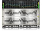
Figure 1: The Graphic Equalizer (Courtesy: https://www.waves.com/plugins/geq-graphic-equalizer)

Types of Equalizers
Graphic Equalizers: Graphic equalizers are the most commonly used equalizers for music systems. It works by allocating a range of frequencies in certain number of bands. The energy in the frequency bands are either attenuated, or boosted, depending on the requirement. The more the number of bands, the more the precision, and vice versa. However, they do not allow control over the shape of the filter for each band. Audio Filters are used to isolate bands, usually in a bell shape around the center frequency.

Parametric Equalizers: These are the most frequently used equalizers in high-end home audio systems and in some recording studios as well. The Parametric Equalizer lets you to control the Center Frequency, its Gain and the Range of each frequency band.

Dynamic Equalizers: This equalizer provides all the facilities given by the parametric equalizers and on top of that provide the user with the control of compression and expansion of an audio signal.

Shelving Equalizers: A shelving equalizer works similar to a High Pass or a Low Pass Filter. Here, the frequencies in the higher or lower end of the spectrum are boosted or attenuated. The boost or attenuation of frequencies is independent of center frequency for a Shelving filter.

Equalizer Fundamentals
In an Equalizer, the audio filters are used to isolate bands around the center frequency, usually, in a bell shape (Band Pass Filter). Analyzing the individual bands of an Equalizer (EQ) yields the filter characteristics of that particular EQ. These are important parameters as they help establish the spectral range in which an equalizer will operate (affect the sound). The filter characteristics are classified into:

Center Frequency: The center frequency for a band establishes the frequency around which the boost or cut in the sound energy affects the audio signal.

Filter Type: Filter Type determine the general shape of the EQ band. The most common filter types that used to design an Equalizer are High Pass Filter (HPF), Low Pass Filter (LPF), Notch Filter, High Shelf Filter (HSF) and a Low Shelf Filter (LSF)

Filter Slope: The slope of a filter indicates the rate of attenuation of sound beyond the cut-off frequency. The filter slope is a term usually associated with band pass, high pass and low pass filters.

Filter Q: It helps determine the bandwidth of a filter band. Q is known as the Quality Factor of an EQ.

Filter Gain: The filter gain is measured in dB (deciBels) and indicates the amount of boost or cut that is applied to a frequency band.

The Architecture of a Typical Equalizer
Almost all modern equalizers are based on Octave based Center Frequencies and use a ‘Frequency Warped’ filter design (i.e. the center frequencies are not equidistant) to minimize the inter-band frequency interference. This results in a smooth transition between bands. The most commonly used Audio EQ has been designed by Robert Bristow-Johnson (RBJ). The RBJ EQ too uses frequency warped time varying digital filters. In a time varying digital filter the filter coefficients change over time. Care must be taken to design the filter coefficients to avoid any noticeable artifacts due to the changing filter coefficients. Switching between one filter response to the other, instantaneously, causes unwanted artefacts in the audio output, hence output crossfading is applied to the nearby bands to reduce the artifacts. Crossfading requires the signal to be filtered with both the old and the new filters in parallel for consecutive bands. Thereafter, to smoothen out the transition in the waveform time-domain based crossfading is applied. The goal of crossfading is to keep the difference between bands to less than 3 dB.

The RBJ filter is an implementation of 2^nd order filters with octave based bandwidth. Since it is an octave based filter, the bands can be divided only w.r.t the octave frequencies, (i.e. 1/3 Octaves or 2/3 Octaves or 1 octave or 2 octaves and so on) and the number of band of the EQ are dependent on the same.

RBJ Cook Book formulae for designing an EQ
A second order filter is also known as a Biquad Filter. The Transfer function for a digital biquad filter (contains two poles and two zeros)

The above equation contains six coefficients. (namely: a0,a1,a2,b0,b1, and b2) The coefficients for the above equation are usually normalized such that a0 = 1. Now we have only 5 coefficients to work with. Since this is an IIR filter, the quantization error in coefficients can lead to instability. To avoid that cascaded second order filters are used in the design. For the filter to be stable, in the Z-domain, all the poles must be inside the unit circle.

Direct Form 1 implementation is typically used for implementing the above transfer function.

Figure 2: Digital Biquad Filter (Image Courtesy: https://en.wikipedia.org/wiki/Digital_biquad_filter)

Using the following “User defined” parameters the appropriate filters can be designed for an EQ.

F_s Sampling Frequency of Audio Signal

f_c Center Frequency of the band

dBGain Used for Peaking and Shelving Filters

Q The Quality Factor

The coefficients for various filters are calculated using the above data and the RBJ cookbook formulae given below:

Low Pass Filter: (This filter removes all the frequencies above a specified frequency. It lets all the low frequencies to pass through and attenuates the higher frequencies)

High Pass Filter: (Removes all the frequencies below a specified frequency. It lets all the high frequencies to pass through and attenuates the lower frequencies)

Band Pass Filter: (Removes all the frequencies above and below specified cut-off frequencies. It only lets the frequencies in a particular band with a lower cut-off and higher cut-off frequency to pass through, and attenuates the frequencies outside the specified band)

Notch Filter: (These work on a very narrow band of frequencies. Removes all the frequencies in a narrow band. Notch filters are a subset a Band-Stop filters, with a very narrow band)

Peaking Filter: (A Peaking filter is used to boost or attenuate a range of frequencies around specified frequencies, to form a bell shape, by a ‘user defined’ value)

Low-Shelf Filter: (A Low-Shelf Filter is used to boost or attenuate a range of frequencies below the specified frequency, by a ‘user defined’ value)

High-Shelf Filter: (A High-Shelf Filter is used to boost or attenuate a range of frequencies above the specified frequency, by a ‘user defined’ value)

Where:
A (gain) = sqrt( 10^(dBgain/20) ) = 10^(dBgain/40) (for peaking and shelving EQ filters only) w0 (Angular freq) = 2*pi*f_c/F_s

alpha = sin(w0)/(2*Q)

Once the coefficients are calculated using the above formulae, appropriate filter functions are called for each band. Usually, Shelving filters (Low-Shelf/High-Shelf) are used for the first and the last band of the EQ and Peaking filters (Bell Filters) are used for all the filters lying in between.

*These are just the fundamental building blocks of an equalizer and in no-way sufficient for designing the equalizer in totality.

Conclusion
Understanding the basics of filter shapes in an equalizer is fundamental to mix or create appropriate sound effects. One needs to know how to use an equalizer properly to make one’s own curves to change the way in which music and movies are heard, completely. Most home audio systems use simple filters for controlling/adjusting bass (low/very low frequencies), mid-range, and treble (high frequencies). When it comes to recording studios, the equalizers tend to be more sophisticated and are capable of finer adjustments. These high-end equalizers are capable of eliminating unwanted noise/sounds, and either suppress certain musical instruments or magnify particular frequencies to make some instruments sound more spectacular.

eInfochips is a CMMi Level 3 & ISO 9001:2008 certified Product Engineering Services company. We at eInfochips create value across the Software Development Life Cycle(SDLC) by providing DSP Middleware Software Development, Porting, Optimization, Support, and Maintenance services for various RISC and CISC SoC’s. We help our customer’s set-up Offshore Development Centers, supplementing the right teams and appropriate execution Models. For more information contact us today.

About the Author
Rhishikesh Agashe holds nearly 19 years of experience in the IT Industry. 4 years as an Entrepreneur and 15 years in the Embedded domain wherein most of his experience was in Embedded Media Processing where he was involved in Implementation of Audio and Speech Algorithms on various Microprocessors/DSPs(ARM/MIPS/TI/CRADLE/CevaDSP/Meta).

References:

Also read:

Understanding BLE Beacons and their Applications

Sign Off Design Challenges at Cutting Edge Technologies

Techniques to Reduce Timing Violations using Clock Tree Optimizations in Synopsys IC Compiler II

Podcast EP10: The M&A Landscape for Semis and EDA

Podcast EP10: The M&A Landscape for Semis and EDA
by Daniel Nenni on 03-05-2021 at 10:00 am

Dan and Mike are once again joined by Dr. Walden Rhines for an overview of the M&A scene for semiconductors and EDA. Wally discusses the periodic expansion and contraction of these markets along with the factors that cause these trends. Wally concludes with a view of the future.

Wally Rhines is widely recognized as an expert in business value creation and technology for the semiconductor and electronic design automation (EDA) industries. https://en.wikipedia.org/wiki/Wally_Rhines

The views, thoughts, and opinions expressed in these podcasts belong solely to the speaker, and not to the speaker’s employer, organization, committee or any other group or individual.

March 5, 2021January 13, 2023

Webinar: Samtec Teams with Otava and Avnet to Tame mmWave Design

Webinar: Samtec Teams with Otava and Avnet to Tame mmWave Design
by Mike Gianfagna on 03-05-2021 at 8:00 am
Categories: 5G, Events, Samtec, Semiconductor Services

mmWave design has traditionally been a boutique technology used in satellite and defense applications. Lately that’s changing. It turns out the complex, high frequency capabilities of mmWave technology are a key enabler for the 5G wireless networks being deployed today. I discussed some of this backstory in a recent post about a new member of the Silicon Catalyst incubator. The design challenges associated with mmWave are substantial. Optimizing the RF signal path is a requirement of course. Dealing with advanced phased-array processing is also a requirement, as is multiple simultaneous beams to deliver low latency with decreasing size, weight, power and cost. That’s why a recent article on Samtec’s website caught my eye. Read on to learn how Samtec teams with Otava and Avnet to tame mmWave design.

There’s a lot of good information on Samtec’s website about mmWave support across multiple applications. There is also an informative webinar coming with Otava, Avnet and Samtec to discuss their collaboration. There are links coming. First, let’s examine the players, the application and the challenges.

Most SemiWiki readers should be familiar with Samtec by now. They provide connectors, cable assemblies and active optical modules across a broad range of applications and performance levels. If you want an introduction to the company, you can find it here. Otava is focused on end-to-end development of technologies used by advanced 5G commercial and DoD applications. Avnet is a leading global technology distributor and solutions provider. The company can support a product at each stage of its lifecycle, from idea to design and from prototype to production.

This is a very interesting collaboration in my view. It is a step above the typical ecosystem work we hear about. The breadth of applications and support offered by these three companies speaks to the daunting requirements for building effective mmWave systems. The beamforming part of the system design is a particularly dauting aspect. Beamforming uses multiple antennas to control the direction of a wavefront by weighting the magnitude and phase of individual antenna signals in an array of multiple antennas. Getting all this right is quite a challenge. Components, interconnect and algorithms all need to work in tight harmony to get the desired result. This kind of technology is what unlocks the high bandwidth and low latency of 5G and its performance is mission critical to many applications, including those found in autonomous driving systems.

The presenters for the webinar include Matt Burns, technical market manager at Samtec. SemiWiki readers should be familiar with Matt. You can hear a podcast with Matt discussing signal integrity challenges here. From Otava, Steve Fireman, senior VP of engineering is presenting. Steve is a co-founder of Otava and has experience designing state-of-the-art RFICs, ICs, module packaging and PCBs related to microwave and millimeter wave phased array systems at Lockheed Martin. Presenting for Avnet is Luc Langlois, director of products and emerging technology at Avnet. Luc has held a variety of roles at Avnet for 15 years and has a broad background in digital signal processing.

The webinar will cover bleeding edge beamformer technology and precision RF interconnect. New evaluation and development platforms that shorten development cycles will also be discussed. If you’re doing any type of 5G development, you should attend this webinar. The webinar was held on March 10, 2021 at 11AM Eastern Standard Time. The good news is that a replay is available. Check it out to see how Samtec teams with Otava and Avnet to tame mmWave design. You can access the webinar replay here. You can also get a broad view of all the 5G network application solutions available from Samtec here.

The views, thoughts, and opinions expressed in this blog belong solely to the author, and not to the author’s employer, organization, committee or any other group or individual.