System-level Electromagnetic Coupling Analysis is now possible, and necessary

With the increasing density of electronics in product enclosures, combined with a broad range of operating frequencies, designers must be cognizant of the issues associated with the radiation and coupling of electromagnetic energy.  The interference between different elements of the design may result in coupling noise-induced failures and/or reduced product reliability due to electrical overstress.

While traditional rules-of-thumb have been very successful in the design of high-speed signals on printed circuit boards – e.g., positioning of ground planes, differential pair impedance matching, route shielding – the complexity of current designs necessitates a much more comprehensive electromagnetic analysis.  It is necessary to incorporate detailed electrical models for passive components, connectors, and (flex) cables, in addition to the (motherboard, daughter, and mezzanine) PCBs, then simulate the electromagnetic response of the system when excited by signal energy of the appropriate bandwidth.

Fortunately, there have been numerous advances over the years in the capabilities to build and simulate full-wave electromagnetic system models.  I recently had the opportunity to review some of these advances with Matt Commens, Principal Product Manager at Ansys, relating to the HFSS toolset.

Introduction

Full-wave computational electromagnetic simulation tools for electronic systems, such as HFSS, attempt to solve Maxwell’s equations for a general 3D environment.  The system is placed in a box that envelops the domain for electromagnetic analysis.  This volume and the electronics within are discretized into a suitable “mesh”.  A large number of (tetrahedral) 3D mesh cells are created, with a denser mesh associated with the detailed, conformal geometries of individual components.

The electric and magnetic fields at the vertices (and the corresponding electric currents across the surfaces) of each mesh cell are represented by a summation of “basis” functions to approximate the solution to the three-dimensional (differential form of) Maxwell’s  equations, at a given frequency of excitation.

A large, but typically very sparse, matrix is generated for the discretized mesh.  The excitation and boundary conditions are specified, and the coefficients of all the basis functions are then solved, providing an excellent approximation to the full system electromagnetic behavior.  Only one matrix solve is needed for all excitations in the system.

Note that this is a fully-coupled electromagnetic analysis, incorporating the material properties and 3D geometry through the discretized volume.

Why is electromagnetic coupling important?  Consider the simple example illustrated above – three examples of a microstrip line on a board are shown, all the same length, but with varying serpentine properties.  Due to the electromagnetic self-coupling present between different segments of the line, the frequency response (e.g., the insertion loss) of each varies significantly –a discretization mesh of the lines with meandering segments is needed to accurately calculate the behavior.

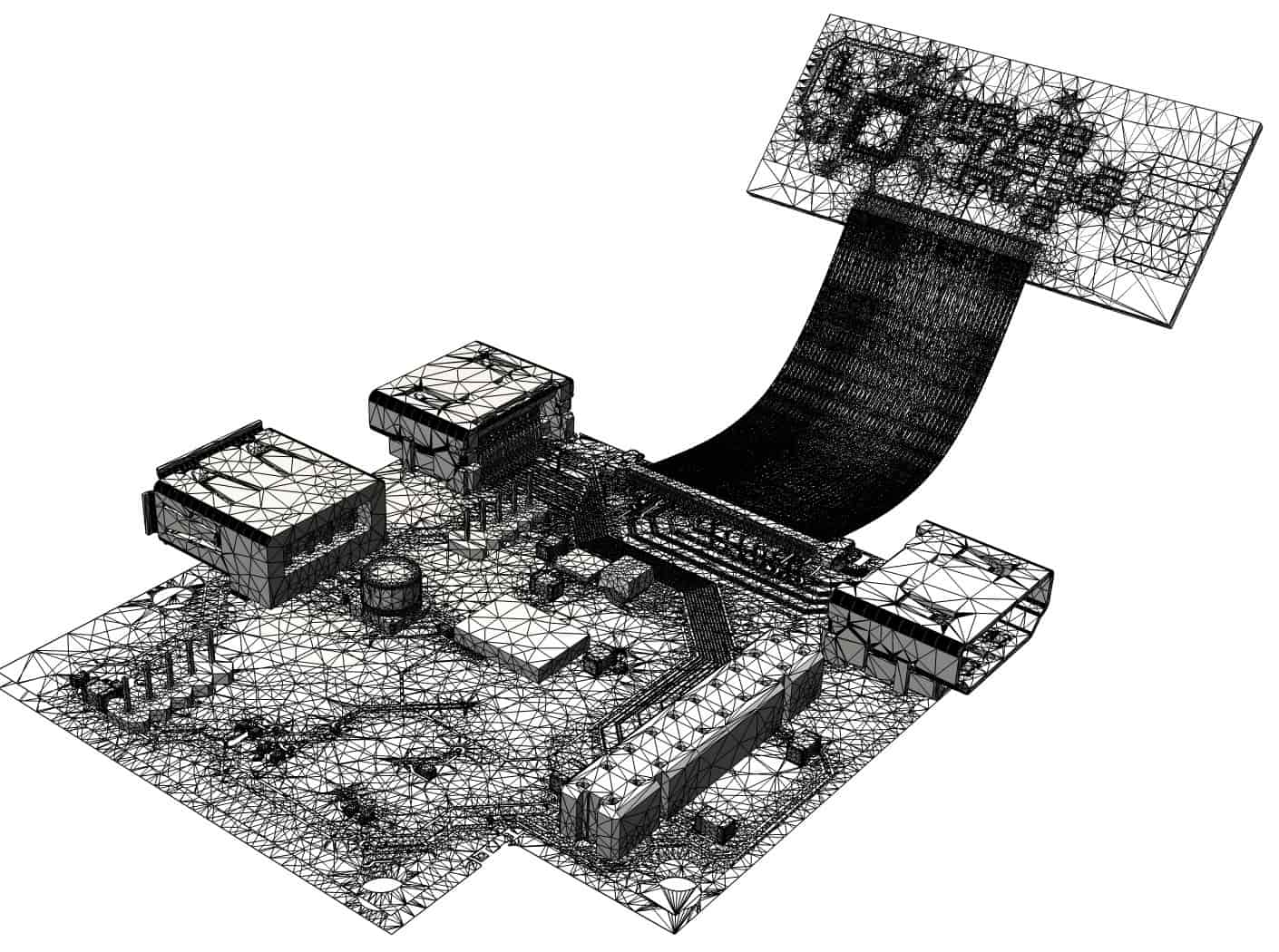
Now consider the example below, where the detailed field distribution is infinitely more complex.  Matt provided this electronic system as a representative example of the types of models for which designers are seeking to analyze the electromagnetic behavior.

Matt chuckled, “When I first starting working with HFSS over 20 years ago, we were solving systems with maybe 10K to 40K matrix unknowns.  Now, we are routinely solving models with more than 100M matrix elements.  The ongoing advances in electromagnetic analysis have dramatically expanded the types of designs that are able to be simulated.”  Matt elaborated on some of those advances.

Computational Electromagnetics

Several algorithmic enhancements have been incorporated into HFSS, to enable the use of HPC resources.

• matrix partitioning and solving across distributed systems

Unique domain decomposition algorithms partition the system-level model (without adding simplifying assumptions at domain interfaces).

• utilization of cloud computing resources, for both the mesh generation and matrix solver
• efficient frequency sweep analysis, across CPU cores and distributed nodes

The broadband frequency response uses an interpolating sweep;  additional sampling points are selected in ranges where the calculated S-parameter response is rapidly changing.

• sensitivity analysis to variations in model parameters (“analytic derivatives”)

This last feature is worth special mention.  Matt indicated, “HFSS supports virtually disturbing the mesh for variation analysis.  Designers can identify a set of parameters in the system model, and readily see how the electromagnetic analysis results change with manufacturing variations, for a small overhead in simulation time, far more efficient than running full simulations on different parameter samples and unique meshes with small dimensional changes.”  This feature provides great insights into where designers could focus on cost versus manufacturing tolerance tradeoffs.

Ansys has prepared an informative demo of how designers can quickly visualize the response to parameter sensitivity – link.

Algorithmic Enhancements for Mesh Generation

Matt identified three key HFSS enhancements of late related to mesh generation.

Adaptive Meshing

The introductory section above described the importance of the 3D mesh to the resulting accuracy.  An initial mesh is solved for the fields – a calculation of the electric field gradient is indicative of where local mesh refinements are appropriate.  (The basis functions for representing the local fields could also be updated.)  A new mesh is solved, and the process iterates until successive passes very less than the convergence criteria.

HFSS recently extended this capability to adapt the mesh each iteration using multiple frequency solutions, over a user-specified range, to enhance the results accuracy when a broad range of spectral energy is present.

3D Components

Traditionally, it has been difficult for designers to build a comprehensive (“end-to-end”) model of even a single long-reach, high-speed signaling interface.  The PCB trace S-parameter model generation from the stack-up was relatively straightforward, but obtaining a model for connectors and cables from the vendor was typically difficult.

Ansys realized that enabling link simulation, and ultimately, system-level analysis required a novel method, and developed the “3D Components” methodology:

• vendors have the tools to generate an encrypted model for release (without applying specific excitations and boundary conditions)
• these “intrinsic” models are simulation-ready

HFSS has full access to the model, but the vendor is able to protect their proprietary IP.

• model re-use is readily supported, through user-defined parameter values (see the figure below)

HFSS Mesh Fusion

Of the steps in the electromagnetic analysis of an electronic system:

• materials specification
• definition of boundary conditions and excitations
• identifying the frequency range of interest
• mesh generation
• matrix solve/simulation, across the range of frequencies
• results post-processing

the key to the final accuracy of the results is mesh generation.  Matt stated, “The optimum meshing approach differs for IC packages, connectors, PCBs, and the chassis – yet, there are coupled fields throughout.  It is crucial to locally use the appropriate mesh technology.”

The combination of adaptive mesh refinement and 3D Component models has enabled Ansys to focus on using the specific meshing technique best suited to the MCAD geometry throughout the system.  The latest Ansys HFSS release incorporates this mesh fusion feature.  Although Matt and I didn’t get a chance to discuss mesh fusion in great technical detail during our call, he indicated there is an upcoming webinar that will go into more specifics – definitely worth checking out.  (Webinar registration link)

Here are the mesh and electromagnetic simulation results from the complex example shown above.

Summary

The traditional method for electromagnetic analysis in electronic systems focused on PCB designs and high-speed signaling.  The board stack-up and materials properties were defined, and the signal traces were simulated.  S-parameter response models for signal loss and (near-end/far-end) crosstalk from adjacent traces were generated, and incorporated into subsequent circuit simulations to measure the overall transmit/receive signal fidelity.  However, the complexity of current electronic systems necessitates a more comprehensive approach to electromagnetic coupling simulation, as compared to concatenating individual S-parameter models.  Systems will be integrating a broad range of signal frequencies from audio to mmWave, with advanced packaging present in aggressive volume enclosures.

The HFSS team at Ansys has focused on numerous technical advances – both computationally and in the critical area of mesh generation – to enable this analysis.  Designers can now evaluate and optimize models of a scope that was once unachievable, with manageable computational resources.

For more info on these Ansys HFSS features, please follow these links (and don’t forget to sign up for the Mesh Fusion webinar):

Broadband Adaptive Meshing – link

Ansys cloud HPC resources – link

3D Components – link1, link2

Mesh Fusion webinar – link

-chipguy

Also Read

HFSS – A History of Electromagnetic Simulation Innovation

HFSS Performance for “Almost Free”

The History and Significance of Power Optimization, According to Jim Hogan

Share this post via:

• 
• 
• 
•