How Fast Can a Performance Model Actually Be Built?

By Thang Tran, CEO of Simplex Micro and Umesh Sisodia, CEO of CircuitSutra

Performance models have a reputation problem. They’re often treated as a long-lead, high-effort undertaking — something a design team commits to early and then waits on for months before it’s useful. The development of SimplEx Micro’s scalar-vector performance model, built in collaboration with CircuitSutra, tells a different story: once the underlying algorithm and methodology are established, extending a performance model to a new microarchitecture is closer to weeks than quarters.

Work began on the performance model in April 2026. By roughly six weeks in, the first-stage model — CPU and VPU pipeline behavior against an idealized cache — was substantially written for microarchitecture validation. By eight weeks in, the model was running real workloads to completion: Dhrystone and a matrix-multiplication (VPU) benchmark, with actual IPC figures being reported rather than projected ones. By twelve weeks in, that wasn’t just running — it was correlated: Dhrystone correlation against RTL was complete, and branch misprediction and L1 cache miss behavior matched RTL trace data exactly.

That’s a functioning, RTL-correlated performance model covering scalar and vector execution in about three months — a timeline more often associated with getting a model started than with getting one validated.

Why Speed Is Possible: A Reusable Foundation, Not a Rebuild

The key to that speed isn’t cutting corners — it’s not starting from scratch. The initial performance model build established a base structure: the modeling approach for pipeline behavior, branch prediction, cache hierarchy, and instruction timing. That structure isn’t specific to one microarchitecture. It’s a methodology that can be ported  a new design and adapted, rather than reinvented.

The important factor is the simplicity of the performance modeling foundation. As anything associated with Simplex Micro, the performance modeling concept is fairly simple in such a way that a new grad who understand computer architecture and C++ programming skill can build a performance model.  The modeling starts with the concept of sharing the instruction decode table between the performance model and the RTL wherein adding or modifying an instruction reflects in both the performance model and the RTL and the correlation effort is significantly less. Similarly, the branch prediction methodology is seamlessly correlated with RTL. The correlation is down the exact cycle of when an instruction is issued in the performance model and RTL.

That’s what makes extending the model to cover new components — like L2 cache behavior and the vector processing unit — a matter of weeks rather than months. With the base structure already proven out, the estimate for adding L2 cache modeling and a full VPU model landed at three to five weeks, with three weeks being the realistic target once the harder architectural questions are worked through early rather than left for later.

Part of what keeps that timeline honest is sequencing: difficult modeling problems get surfaced and discussed immediately, rather than discovered late. If something proves genuinely hard to implement, that gets flagged and, if it’s not critical to the near-term milestone, deliberately deferred — not silently absorbed into a slipping schedule. Anything considered low-importance and high-difficulty gets pushed to a later phase explicitly, keeping the core timeline intact instead of blocked on edge cases. By-the-way, these cases are rare and not common cases.

This is the same discipline visible in the benchmark rollout: Dhrystone, then matrix multiplication, then TinyML and Qwen, added one at a time, with correlation against RTL chased down benchmark by benchmark rather than declared complete in aggregate. It is not correlating that the IPC and the ratio numbers, but the actual cycle-by-cycle correlation.

The Payoff: A Demo-Ready Model, Fast

The practical result of this pace is that the performance model isn’t just a research artifact by the time it’s shown externally — it’s a working tool that already covers the full compute engine: scalar, and vector, validated against real benchmark workloads including TinyML and Qwen. That’s a meaningfully different pitch than “here’s our roadmap” — it’s “here’s a model you can point your own workload at today.”

Speed only matters if the result is usable by someone other than the team that built it. The model doesn’t come back as a black box with results attached — it ships with documentation that lets a design team run it themselves. That’s a meaningful distinction from the RTL alternative it’s meant to complement: exploring a configuration change in RTL means going back to whoever owns the re-synthesis flow and waiting on a multi-day turnaround. With a documented, self-service performance model, a design team can test a cache size or issue-width change on their own, in minutes.

That’s the same value proposition as the model’s speed of development, applied downstream: a tool built quickly is only useful if it’s also built to be handed off.

Beyond Numbers: Seeing the Pipeline, Not Just Measuring It

Most performance models stop at the aggregate: an IPC number, a cycle count, maybe a stall breakdown by category. That’s useful for tracking a target, but it doesn’t tell a design team why a particular region of code is slow, or which of several overlapping issues is actually responsible for a dip. SimplEx Micro’s performance model pairs its correlation work with a visualization layer built to close that gap.

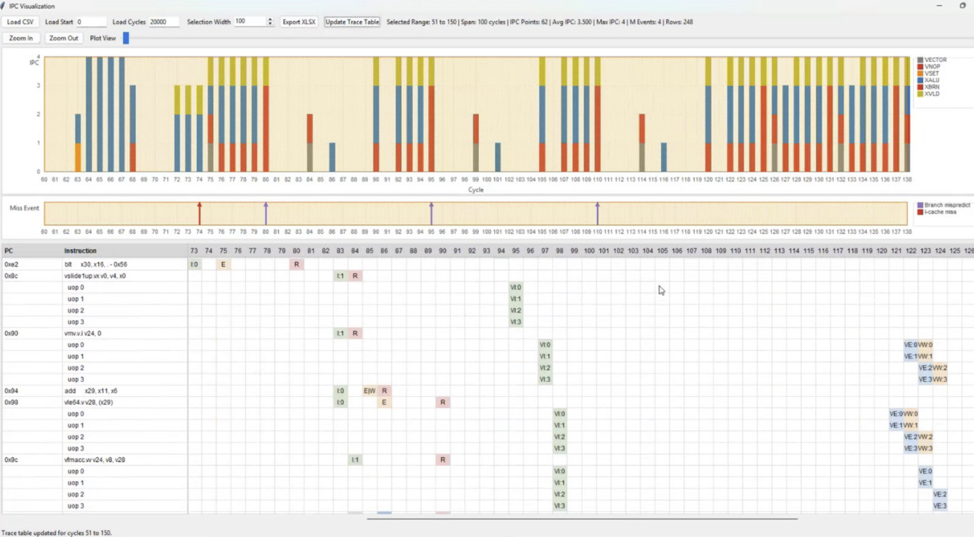
The IPC Visualization tool, shown below, plots per-cycle IPC across an entire run and a dynamically color-coded instruction classes — ALU, branch, vector, vector load, vector store, CSR, divide, load, multiply, store — so a design team can see at a glance where execution is scalar-bound, vector-bound, load-bound, or branch-heavy. A dedicated miss-event track sits directly beneath it, flagging D-cache misses and branch mispredictions cycle by cycle, including cycles where both occur in the same cycle. The IPC plots can be zoom in or out and selecting any range of cycles drills straight into a trace table showing, instruction by instruction, exactly when each instruction was issued, executed, written back, and retired, down to the specific PC. The vector instruction includes the micro-operation for each VRF results. The instruction pipeline can be saved into an excel file for review at later time.

Why This Matters for RISC-V IP Designers

For designers evaluating RISC-V IP, the speed of the performance model isn’t a side detail — it’s part of the value proposition. Our performance model uses the RISC-V open-source compiler and Whisper Instruction in which any design team can use with the right c library and Linux version.  A model that can be extended to new configurations in weeks, not quarters, and then handed to a design team to run independently, is a model that can actually keep pace with designers’ own design exploration. It’s the difference between a performance model as a static deliverable and a performance model as a living tool that evolves alongside the architecture it’s describing.

Also Read:

CEO Interview with Dr. Thang Tran of Simplex Micro

AION Silicon: Architecting Smarter SoCs with RISC-V: Balancing Performance, Flexibility, and Risk

RISC-V and AI: The Architecture Shift Is Now