Ultra-low Voltage: Is Your Slack Really Positive? Are You Sure?

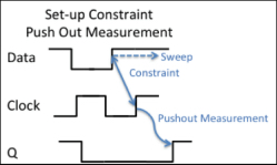
During synthesis and static timing the main figure of merit is “slack”. If a signal arrives with time to spare before it is needed (often measured against the setup time before a clock changes at a register) then the slack is positive. Positive slack is generally a good thing, although it can indicate over-design if it is large. If a signal arrives late then the slack is negative. Obviously, the goal for signoff is to have all slack positive or zero.

Signal timing is actually measured against timing constraints. These come from two sources. One is the user who can specify things like the clock frequency or timing limits at output pins. These basically let the user express the desired behavior of the design. The other source is the cell library where the characterization data is captured. Particularly important are the setup and hold times for flipflops and latches. A further complication is that these checks need to be performed at several process “corners”, traditional ones such as FF and SS but for a modern process, at many other temperature, voltage and process conditions too.

Measuring slack for ultra-low voltage operation—below 0.7V—brings additional challenges, especially process variance. Paths that appear to pass timing within a corner may fail when process variance is included. Even at older process nodes such as 55nm or 65nm, process variance within a PVT corner can show up when the threshold voltage is severely reduced.

The set-up and hold timing checks that are pre-characterized for flip-flops, latches and registers in a cell library are especially vulnerable to variation. Process variance has as much impact on the timing constraints as it does on delay variation. In fact, the corner timing constraints for lower voltages may be extremely optimistic and hide timing violations. They are overstating the timing slack in the design.

During the medieval ages of chip design the solution was always to trade off any lack of accuracy with pessimism. How bad can it be? Use that number. But in a modern process, that doesn’t work. Often it will prove impossible to close timing with “that number” because there isn’t enough timing headroom to waste a lot of it on pessimism. Plus “that number” varies depending on corner, temperature, load, slew-rate and so on. Lack of accuracy has to be fixed by increasing accuracy.

The Liberty Variation Format (LVF) supports an approach known as constraint uncertainty. This adjusts the timing constraints to reflect the impact of process variation on a very granular basis: each slew/slew constraint condition gets a unique value. Constraint uncertainty makes sure that margin gets added in exactly the right places, and with the level of conservatism the user specifies to protect against critical set-up and hold violations. By combining constraint uncertainty with arc/load/slew specific delay variance (also supported by LVF) engineers can close timing with much higher confidence and precision. There are other approaches, such as adding values direct to the .lib timing library, but they suffer from various limitations.

Timing constraints, like the delay tables for the libraries, have traditionally been characterized at the process corners: SS and FF. They do not use the global corners SSG/FFG and then add in local on-die variance. However, process variation can affect the transistors inside of a flip-flop or latch just as much as they do the gates along a data or clock path. Engineers are often shocked to see that delay can swing by as much as 2X or more on a cell because of process variation.

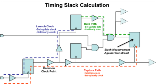
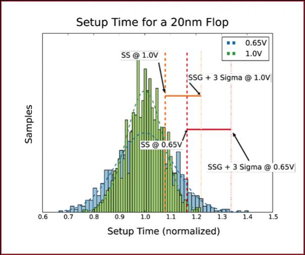For example, the diagram above shows the setup constraint for a 20nm flipflop measured at 1V (in green). It also shows the constraint measured at the SS corner (one of the places where cells are normally characterized) versus SSG+3σ (the red vertical dashed lines). There is considerable pushout, the constraint is optimistic. Turning to the 0.65V characterization (in blue) there is an even larger pushout (to the red dotted line). The constraint is very optimistic and so will overstate slack. What looks like a reassuring positive slack may well be negative slack, a recipe for a chip that doesn’t work.

There are two approaches to generating constraint uncertainty values: Monte Carlo (MC) SPICE or CLKDA’s Variance FX. All of the MC SPICE based approaches depend on sampling. Simulating a flip-flop is time consuming at best; simulating it 100’s of times or 1000’s of times for accuracy at low voltage, can be prohibitively slow. Variance FX, the industry leading solution for variation characterization can be hundreds of times faster than MC SPICE. The FX model and simulator solve for variance without any sampling and are typically within ± 2% of MC SPICE for nominal ± 3σ. Variance FX supports the classic approaches for constraint uncertainty, and has multiple options for characterizing constraints efficiently.

The bottom line: traditional corner based constraints are very optimistic, and will overstate timing slack. Paths that appear to be passing may be failing, and by a lot. Positive slack may be negative. Working chips may…not.

The CLKDA white paper The Impact of Process Variance on Timing Constraints and Slack at Ultra Low Voltage is here.