My first introduction to modeling an AMS behavior using a language was back in the 1980’s at Silicon Compilers using the Lsim simulator. Around the same time the VHDL and Verilog languages emerged to handle the modeling of both digital and some analog behaviors. The big reason to model analog behavior with a language is for improved simulation speeds to boost productivity of both the design and verification phases, but the challenge is to consider the trade-off in accuracy versus a reference like SPICE circuit simulation.
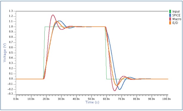
Pulse response of an Operational Amplifier:SPICE in blue, Real Number model in Orange
Coming from a circuit design background I have come to trust the accuracy of SPICE because it models and simulates quite closely to silicon behavior for DC, transient, voltages and currents of both MOS devices and interconnect on analog designs. But who wants to wait one week for a large AMS block to simulate when running SPICE?
One technique to speed up analog and AMS simulation speeds is using Real Number (RN) modeling, where the simulator uses an event-driven approach. When using RN modeling, first ask yourself if the desired behavior fits within the following limitations:
[LIST=1]
AMS Modeling Abstraction
There are two popular approaches to abstracting AMS models today:
- AMS modeling with VHDL-AMS, Verilog-A and Verilog-AMS where each transistor uses a behavioral model, reducing simulation times. Up to 100X simulation speed-ups over SPICE are typical.
- RN modeling with an event-driven algorithm for analog components, where time is discrete and the simulator manages events, not equations. Up to 1,000X simulation speed-ups over SPICE are possible.
RN Model Limitations
Going back to our initial list of limitations for RN modeling, #1 states that a RN model can be written for the voltage or the current on one net, but not both at the same time. Limitation #4 says that you must model the behavior with an explicit solution to the equations.
Since RN modeling uses an event driven approach, while analog signals are continuous in nature there is a requirement with RN simulation to approximate the continuous signals using polynomial functions like Piece Wise Constant (PWC) or Piece Wise Linear (PWL) techniques.
With an Analog HDL you can have coupling between models, however with RN modeling the coupling between different models is not allowed.
For some linear systems you can model the analog function as a Laplace transform, making it possible to describe the output as a function of: inputs, their history, and the history of the output. You do this by transforming the Laplace filter into a Z transform by sampling both the input and output signals at a sampling frequency: The math looks like:

S is the complex frequency operator, and T is the sampling period. T needs to be high enough for accurate results, yet low enough to keep simulation speeds fast.
Event-Driven Languages
We are fortunate to have three language choices supporting RN modeling: SystemVerilog, VHDL-AMS and Verilog-AMS with the wreal extensions. The following table shows how each of these languages support modeling features:
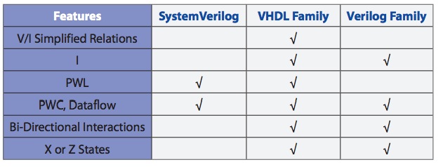
While writing your RN models, there will be continual validations versus your reference SPICE circuit simulator.
Engineers have been writing RN models for a few decades now, and it’s recommended to use RN for analog when:
- You don’t need a conservative system with data flow models.
- Using conservative models only for the voltage or current.
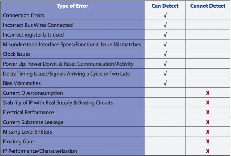
RN modeling can catch many typical design errors, but not all:
RN Modeling Example
Our first waveform in this blog article showed the response of an operation amplifier as described with RN models. That design was selected because we can code the OpAmp equations as a function of the inputs and its history, plus the history of the output. You start out running SPICE with an AC analysis, noting the two pole response as the golden reference:
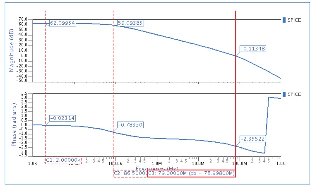
AC response of a SPICE OpAmp using Questa ADMS from Mentor Graphics
The two dominant poles were measured at 86.5 kHz and 79.0 MHz, and you can then plug these two values into a macro model and simulate with a SPICE simulator like Eldo, from Mentor Graphics.
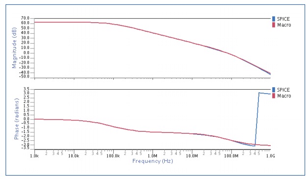
AC comparison with SPICE and macro model amplifiers
The OpAmp equations with two poles are modeled using:


We then want to model the closed loop gain, which is related to open loop gain as:

The final transfer function is described as:

Coded in Verilog-AMS with wreal this looks like:
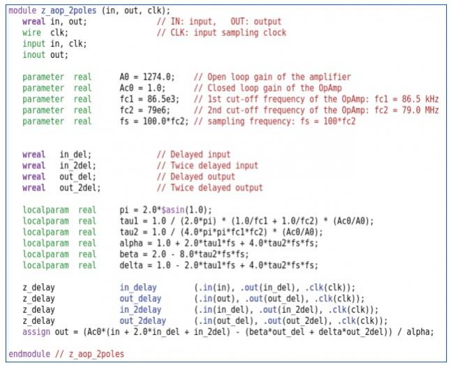
Simulating the various models and then comparing them versus SPICE:
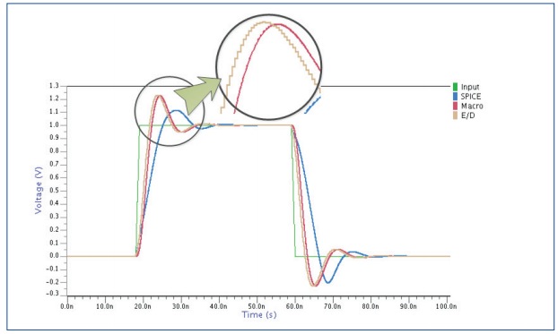
Results from the macro model in Red track with the RN model in gold, however they aren’t matching the SPICE results in blue. This simulation mismatch is caused by the output slew rate of the amplifier. By adding extra RN code to account for slew rate, the new simulation results are much closer to SPICE:

A comparison of simulation speeds showed that RN modeling was 54X faster than SPICE without the slew rate effect, and 42.5X faster with the slew rate effect.
Summary
Simulation times for AMS circuits can be sped up by using RN modeling techniques, while maintaining acceptable accuracy levels. Your team just needs to be aware of where RN modeling is appropriate.
Further Reading
The engineers at Mentor Graphics have authored a 16 page White Paper, Event-Driven (RN) Modeling for AMS Circuits, available for download here. They also showed the pitfalls of applying RN modeling to a 2nd order sigma-delta modulator.
lang: en_US
Share this post via:


Comments
0 Replies to “Speeding Up AMS Verification by Modeling with Real Numbers”
You must register or log in to view/post comments.