Chapter 1 – Predicting Trends in the Semiconductor Industry

Figure 1 is the most basic of all the predictable parameters of the semiconductor industry, even more so than Moore’s Law.  It is the learning curve for the transistor.  Since 1954, the revenue per transistor (and presumably the cost per transistor, if we had the data from the manufacturers) has followed a highly predictable learning curve.  Before Moore’s Law, the learning curve provided a guiding light for the semiconductor industry.  Texas Instruments used it for strategic advantage and shared its data with Boston Consulting Group who published a book called “Perspectives on Experience”¹.  In the days of germanium and silicon discrete transistors, companies like TI could use the learning curve, for example, to predict what the unit cost would be after 100,000 units were produced, based upon the actual cost per unit of the first 1,000 units produced.  They could then price the particular transistor product at a loss initially to gain leading market share and therefore achieve higher profitability and market influence when they reached future high unit volume sales.  TI didn’t create the technology of learning curves.  It was developed in 1885² and has been used in industries like aviation, even before the transistor was invented, to predict the future cost per airplane when a certain cumulative unit volume was achieved.  TI’s unique approach for semiconductors lay in the use of the learning curve to drive a

pricing strategy early in the life of a new component.

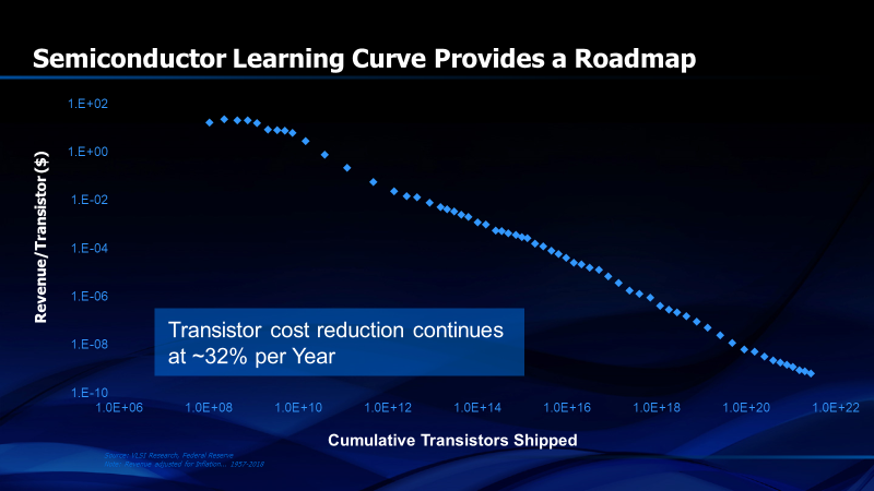
Figure 1.  Learning curve for the transistor from 1954 to 2019

Figure 2 shows how the learning curve works.  The vertical axis is the logarithm of the cost per unit of anything that is produced.  The product can be a good or service; anything that benefits from the experience of doing the same thing, or making the same product, again and again.  Published learning curves typically use the revenue per unit because companies are unwilling to divulge their cost data.  The companies, however, know their costs and, over the history of the semiconductor industry, have used that data to strategically position themselves against competition.  The horizontal axis of the learning curve is the logarithm of the cumulative number of units of a product or service that have been produced throughout history. When the data is plotted, it results in a straight line with a downward slope.  Cost per unit decreases monotonically as we develop more experience, or “learning”.  Since the learning curve is a “log/log” graph, the data generates a line rapidly initially as the small number of cumulative units doubles in a short period of time.  As time goes on, movement of the straight line to the right slows since it takes longer to double the total cumulative number of units.  Every time the cumulative number of units produced doubles, the line reflects a decrease in the cost per unit by a fixed percentage.  The percentage is different for different products but tends to be similar across a broad range of products in an industry like semiconductors.

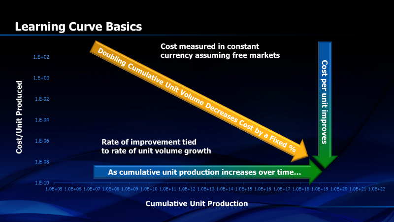
Figure 2.  The learning curve is a log/log plot of cost per unit vs cumulative units manufactured

More broadly, learning curves can be applied to any good or service where the cost per unit of production can be measured. We are just not as aware of the phenomenon today because the measurement applies only when cost is measured in constant currency.  A deflator must therefore be applied to the cost numbers to account for the portion of inflation that is caused by governmentally driven inflation.  In addition, the learning curve only applies in free markets. Tariffs, trade barriers, taxes and other costs must be removed before actual cost comparisons can be made.  The reason that learning curves have been so valuable in the semiconductor industry is that it is one of the few industries that has operated for over sixty years in a relatively free worldwide market, with minimal regulation and tariffs as well as a very low cost of freight between regions.

One of the great things about semiconductor learning curves is that they will be applicable as long as transistors, or equivalent switches, are produced. While Moore’s Law is quickly becoming obsolete, the learning curve will never be.  What will happen, however, is that the cumulative number of transistors produced will stop moving so quickly to the right on the logarithmic scale.  Then the prices will not decrease as rapidly as they have in the past. The visible effect of improved learning will diminish.  At some point, monetary inflation will be larger than the manufacturing cost reduction and transistor unit prices may actually increase with time in absolute dollars even though they are decreasing in constant currency. In the meantime, the learning curve is a useful guidepost for predicting the future. Currently, in 2019, the revenue per transistor is decreasing about 32% per year.

Those who purchase microprocessor or “system on chip” (SoC) components may recognize that, in 2017, the price per transistor is decreasing at a slower rate than 32% per year. Figure 3 explains this. The 32% number applies to the total of all semiconductor components produced in 2017. However the cost per transistor is made up of different kinds of semiconductor components — memory, logic, analog, etc.  It becomes apparent from Figure 3 that the semiconductor industry is producing far more transistors in discrete memory components, particularly NAND FLASH nonvolatile memories, than in other types of semiconductors.  When the memory learning curve (consisting mostly of NAND FLASH and DRAM) is separated from the non-memory learning curve, it is evident that cost per transistor and cumulative unit volume for memory are way ahead of non-memory.  That’s okay because the learning curve doesn’t specify how the decreasing cost per transistor is achieved – only that it will happen as a function of cumulative transistors produced.

Figure 3.  Cumulative unit volume of transistors used in memory components is increasing much faster than unit volume of transistors in other types of chips.

Another aspect of interest in Figure 3 is the set of data points near the end of the curve that were generated by data from 2017 and 2018.  The data points are above the learning curve trend line. How can this happen if the learning curve is a true law of nature?  Very simply, the period from 2016 through 2018 was one of memory shortages, particularly DRAM.  Prices per transistor increased instead of decreasing because market demand exceeded supply.  Won’t this cause a long- term deviation from the learning curve?  No.  Whenever a market supply/demand imbalance occurs, the cost per transistor moves above or below the long-term trend line of the learning curve.  This is always a temporary move.  When supply and demand come back in balance, the cost per transistor will move to the other side of the learning curve.  Area generated above the learning curve will normally be compensated by a nearly equal area below the learning curve and vice versa.  This is another useful benefit of the learning curve because it allows us to predict the general trend of future prices even when short term market forces cause a perturbation.

While I’ve focused on transistors in this discussion of learning curves, it should be noted that we could just as easily use electrical “switches” as our unit of measure.  The same learning curve would then work for mechanical switches, vacuum tubes and transistors as seen in Figure 5 of Chapter 3.  This figure also shows another attribute of the learning curve.  In this case, the metric on the vertical axis is revenue per MIP (or millions of computer instructions per second) for various types of electrical switches.  Learning curves can be used to predict improvements in performance, reliability (in FITS), power dissipation and many other parameters that benefit from the cumulative unit volume of production experience.

Learning curves also provide a useful tool for predicting “tipping points” for new technology adoption.  A good example is the introduction of “compression technology” in the semiconductor test industry in 2001.  In hindsight, a major innovation like this was inevitable just by examining the learning curve for the cost of testing a transistor in an integrated circuit (Figure 4). The ATE cost learning curve was not parallel to the silicon transistor learning curve and had a less steep slope.  Industry ATE cost was not decreasing fast enough.

The ATE industry should have seen that change was inevitable.  Pat Gelsinger, in his Design Automation Conference Keynote address in 1999 highlighted his prediction that “in the future, it may cost more to test a transistor than to manufacture it”.  Such a prediction would have occurred had it not been for compression technology (also called “embedded deterministic test”) which started out in 2001 with a 10X improvement in the number of “test vectors” required to achieve the same level of test and then progressed to nearly 1000X by 2018³.

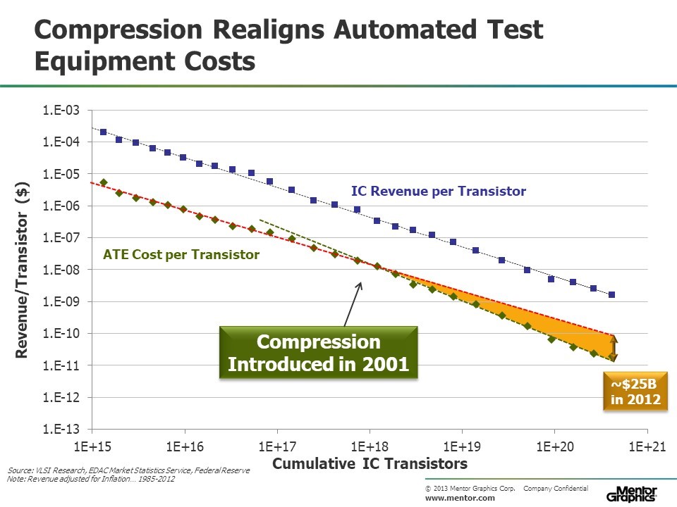
Figure 4.  Until 2001, reduction in the revenue per transistor of the automated test equipment industry was decreasing at a slower rate than the transistors produced by their customers, the semiconductor component industry.

Introduction of “embedded deterministic test”, or test compression, in 2001 significantly reduced the number of testers required and, by 2012, reduced the revenue of the ATE industry by $25B per year.

 

¹ Boston Consulting Group, “Perspectives on Experience”, 1970, Boston, MA

² https://en.wikipedia.org/wiki/Learning_curve#In_machine_learning

³Rajski, J., Tyszer, J., Kassab, M. and Mukherjee, N., “Embedded Deterministic Test”, IEEE Transactions on Computer-Aided Design of Integrated Circuits and Systems ( Volume: 23 , Issue: 5 , May 2004

Read the completed series

Share this post via:

• 
• 
• 
•