Path FX – the Production Proven Answer to Static Timing Analysis with Variation

I want to compliment ChipGuy on a very nice write-up of a complex topic – how to model process variation in static timing.

The Latest in Static Timing Analysis with Variation Modeling

For those who are interested in more depth on this topic, you should refer to the CLKDA SemiWiki section. There are multiple articles on this topic HERE.

CLKDA’s Path FX, our Monte Carlo (MC) SPICE accurate, transistor level timing solution, is the only commercial, production proven timer that currently addresses the challenges ChipGuy outlined, specifically non-Gaussian delays. Our customers are using Path FX to achieve MC SPICE accurate timing in 16nm, 14nm and 10nm processes, at 0.5V and below. Path FX’s non-Gaussian accuracy has been verified in actual silicon on multiple designs, not just 40 selected paths.

I would like to clarify a few points in ChipGuy’s article, particularly with respect to his analysis of the product datasheet Cadence recently presented at TAU. First, I would like to bring the discussion up a level, and then, because this is static timing, dive right back into the weeds.

“Recovering Margin.” This is the #1 timing methodology goal at our leading edge customers. The silicon data is there. The current STA practices over-margin to the detriment of power, area, timing closure, and time to market. In today’s highly competitive chip markets, this is a recipe for disaster.

ChipGuy hits the bull’s-eye at the beginning of his article. The existing “static timing analysis (STA) is more of an art than a science” that requires too many fudge factors that consume margin, and he mentions SI, IR, jitter… as contributors.

However, ChipGuy misses the elephant in the room, and the fundamental limitations of Cadence’s approach. PrimeTime and Tempus force a trade-off: performance vs. accuracy. In order to evaluate big designs, they require black box models like CCS, or ECSM, factors like AOCV, or SOCV. Even with Cadence’s elaborate addition of more statistical moments to the characterization flow, their methodology is at best an approximation for both delay and variation.

Now back down into the weeds.

The highest accuracy analysis tool for pre-silicon timing is MC SPICE.It is not viable for looking at millions of paths, but it is the benchmark.

And the ultimate metric is statistical slack: how much does each path pass or fail by when all of the process variation is taken into account. Statistical slack is the metric that combines all off the process variation impact on arrival times, set-up and hold checks, and slews into one number.

MC SPICE accurate statistical slack is also the best standard for recovering margin! By getting timing (delays, constraints, slack) as close as possible to MC SPICE, margin factors can be dramatically reduced.

Now the Cadence proposal, with its costly characterization of even more data for every cell/arc/load/slew, only addressed one part of the MC SPICE slack equation – arrival times. Their proposal is missing all of the other critical values: statistical slews correlated with delays at each node, statistical common clock pessimism removal, non-Gaussian timing constraints, and the correct probability evaluation at the endpoint. In fact, our data shows that on some paths statistical slew can have as big an impact on slack as delay variance.

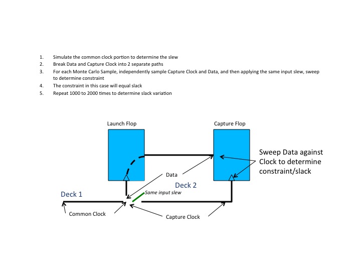
Lets look at how MC SPICE solves for statistical slack. There are no pre-characterized constraints, libraries or delay models. There is just the circuit. MC SPICE has to evaluate every sample to see if it passes or fails (did the value get latched in). Then for every passing sample, it sweeps that sample to determine the slack (how much did it pass by). After running thousands of samples, you get a statistical distribution for slack, as well as all of the constituent values you would expect to see in an STA approach (arrival times for clock and data). The result will be the average and the distribution whether it is Gaussian or non-Gaussian. MC SPICE does not care.

Here is one methodology for using MC SPICE to measure statistical slack.

What is immediately apparent is that Cadence is only addressing at best one third (maybe less) of the problem. With their new SOCV scheme that adds in all of the moments, they have an approximation for non-Gaussian arrival times. What’s missing is all of the other key elements: statistical slew, non-Gaussian constraints, etc.

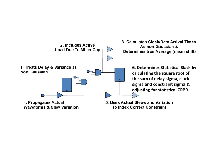
Path FX, by way of contrast, incorporates all of these elements with MC SPICE accuracy. In a recent test on hold side, ultra-low voltage test paths at 0.5V at 10nm, Path FX was within 1% of MC SPICE for average and sigma for clock and data arrival, the hold constraint, slack and statistical slack. Everything, including delays and constraints, were non-Gaussian!

When Path FX calculates statistical slack, it combines both the delays and the variances to properly model statistical cancellation. The correct statistical operation (the root of the sum of the squares of the sigma’s for delay, clock and constraint) to determine statistical slack is as follows (adjusted refers to statistical CRPR).

𝑆𝑖𝑔𝑚𝑎𝑠𝑙𝑎𝑐𝑘= (𝑎𝑑𝑗𝑢𝑠𝑡𝑒𝑑_𝑎𝑟𝑟𝑖𝑣𝑎𝑙_𝑠𝑖𝑔𝑚𝑎2+𝑎𝑑𝑗𝑢𝑠𝑡𝑒𝑑_𝑟𝑒𝑞𝑢𝑖𝑟𝑒𝑑_𝑠𝑖𝑔𝑚𝑎2+𝑐𝑜𝑛𝑠𝑡𝑟𝑎𝑖𝑛𝑡_𝑠𝑖𝑔𝑚𝑎2) 1/2

Most importantly, because Path FX is transistor level, it does not require special characterization for skew, kurtosis, or mean shift. AND Path FX has the same or better performance and capacity as the leading STA tools. Moreover, the FX model is generated directly from the Foundry BSIM models in minutes, instead of needing days or weeks to characterize.

To learn more about how Path FX calculates statistical margin, check out this white paper HERE:

To learn more about how Path FX can help you recover margin, visit us at:http://www.clkda.com

Share this post via:

• 
• 
• 
•