

(Adapted from a presentation first given under this title in 1989 and subsequently expanded in presentations over a period of nearly thirty years)
In 1965, Gordon Moore, then R&D Manager for Fairchild Semiconductor, published a paper in “Electronics” magazine predicting the trend for semiconductors in the next ten years. He showed a graph of the number of components in the largest chips in each of the last four years that followed a straight line when plotted with a Y-axis that was the base two logarithm of the number of components (transistors, capacitors, resistors or diodes) and the horizontal axis was time. The number of components had doubled every year (Figure 1). This graph became known as “Moore’s Law” and has been extrapolated for more than fifty years. It is not a “law”. It is an empirical observation that became self-fulfilling after some adjustments.
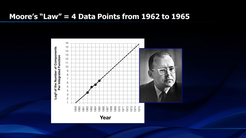
Figure 1. First presentation of Moore’s Law in 1965
Ten years later, in 1975, Gordon Moore revised “Moore’s Law”, saying that the doubling of transistors per chip was now occurring every two years, instead of every year. Then, in 1997, Gordon Moore revised “Moore’s Law” once again, showing that the doubling of transistors was now occurring every 18 months. These repeated revisions affirm that “Moore’s Law” was not actually a law of nature but an interesting, if temporary, phenomenon. In science and engineering, we have laws that predict outcomes when variables change, like the first and second laws of thermodynamics, Newton’s laws of motion or Maxwell’s equations. They don’t change over time, unlike Moore’s Law (Figure 2). Even Dr. Moore pointed out, in his ISSCC keynote in 2003, that “no exponential is forever”.
Why did “Moore’s Law” take on such significance and work so well, despite the adjustments in time scale? The answer is that “Moore’s Law” is based upon an actual law of nature called the “learning curve” (See Figure 1 in Chapter 1). Learning curves have been used over the last hundred years to predict the future cost per unit of products as diverse as airplanes, beer and transistors. They were used strategically by Texas Instruments in the 1960’s to “forward price” new semiconductor components in order to achieve a desired future market share and profitability.
The learning curve and Moore’s Law are actually the same when two conditions are met. These are: 1) If most of the cost reduction for semiconductor chips comes from shrinking feature sizes and growing wafer diameters and 2) If the cumulative number of transistors manufactured by the semiconductor industry increases exponentially with time. If these two conditions are met, then Moore’s Law and the learning curve become straight lines that predict the same trend (Figure 3).
If “Moore’s Law” is based upon a real law of nature, i.e. the learning curve, then why did it have to be adjusted from one year to two years and then back to eighteen months? The answer comes from assumption number two above and is shown in Figure 4. Even though the number of transistors shipped each year has grown exponentially through most of the history of the semiconductor industry, there was a period when growth slowed and then later returned to the exponential trend. That change in growth rate caused “Moore’s Law” to increase from one to two years and then back to eighteen months. Because the learning curve is a log/log graph, exponential growth of the cumulative number of transistors produces a straight line with time as well as with the cumulative number of transistors. Unlike Moore’s Law, the learning curve works well even if the exponential growth of units deviates. Moore’s Law uses time as its horizontal axis so linearity is assured only if cumulative transistor growth is exponential.
Today, many people worry that the inevitable end of Moore’s Law will leave us with a stagnant semiconductor industry with no guideposts to drive new silicon technology directions. Fortunately, these people need not worry. The learning curve is valid forever (when measured in constant currency, corrected for governmentally-induced inflation) as long as free market economics prevail, i.e. negligible trade barriers, no regulatory price controls, etc.
Figure 5 shows a learning curve for the electronic switch measured as revenue per MIP, beginning with vacuum tubes and progressing through germanium and quickly transitioning to silicon. We use industry revenue for the vertical axis, instead of cost, because the data is more readily available but the two variables should be surrogates for one another. The horizontal axis is the cumulative number of transistors shipped throughout history. That number has been available from the Semiconductor Industry Association, as well as from other semiconductor analysts, for decades.
Of course, the learning curve for electronic switches doesn’t care whether the cost reduction is achieved with mechanical switches, vacuum tubes, transistors or even carbon nanotubes in the future. The learning curve is technology independent if a more generalized unit than transistors is measured. We therefore have a metric to track when the further improvements in cost or power are so difficult with silicon that we have to consider an alternative like carbon nanotubes or bio-switches. The important result of this information for the electronics industry is that the death of Moore’s Law doesn’t lead to random, unpredictable trends in semiconductor technology. We have a road map. As long as we can measure the growth rate of transistor shipments, we will know the cost or revenue per transistor of the semiconductor industry, or vice versa.
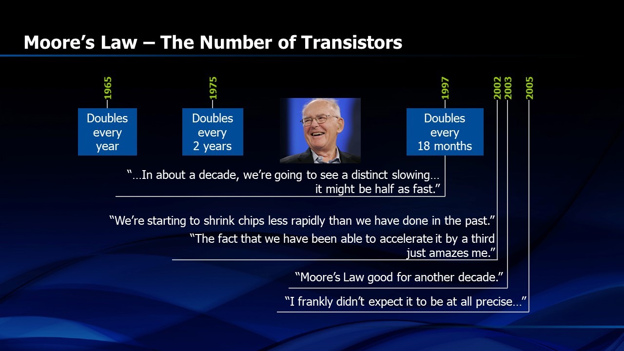
Figure 2. Moore’s “Law” evolved over time
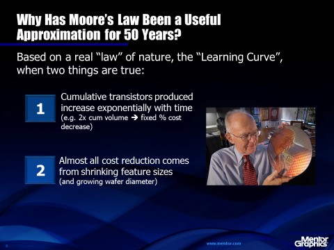
Figure 3. Learning Curve and Moore’s Law are the same under certain conditions
![]()
Figure 4. Growth in cumulative number of transistors has not always been exponential with time
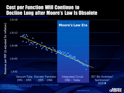
Figure 5. Cost per Function, or per MIP, transcends the transistor era
Share this post via:


The Packaging PDK Is the Missing Layer for Co-Packaged Optics