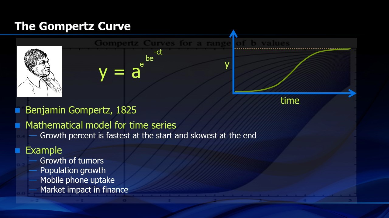


In 1825, Benjamin Gompertz proposed a mathematical model for time series that looks like an “S-curve”.1 Mathematically it is a double exponential (Figure 1) where y=a(exp(b(exp(-ct)))) where t is time and a, b and c are adjustable coefficients that modulate the steepness of the S-Curve. The Gompertz Curve has been used for a wide variety of time dependent models including the growth of tumors, population growth and financial market evolution.
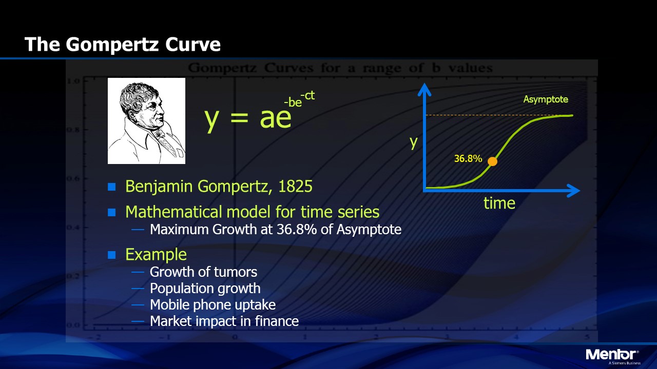
FIGURE 1. The Gompertz Curve
S-Curves are common in nature. In any new business, or in biological phenomena, we start out small with an embryonic business or a tiny cell and it reproduces slowly but the percentage growth rate is large. As time goes on, the growth accelerates until it finally slows down as it reaches saturation. A new product takes a significant period of time for early adopters to spread the word of its benefits but it then goes viral, saturates the market and then declines (Figure 2). On the right half of Figure 2, we see the same phenomena when the vertical axis of the graph is the cumulative number. An example would be the freezing of water in a pond. It starts with a few water molecules and then grows to a critical nucleus which grows rapidly until the pond is mostly frozen. Then the last bit of water freezes over a longer period of time. Expressed mathematically, the integral of the cumulative function is the area under the curve and it increases until the S-Curve finally flattens.
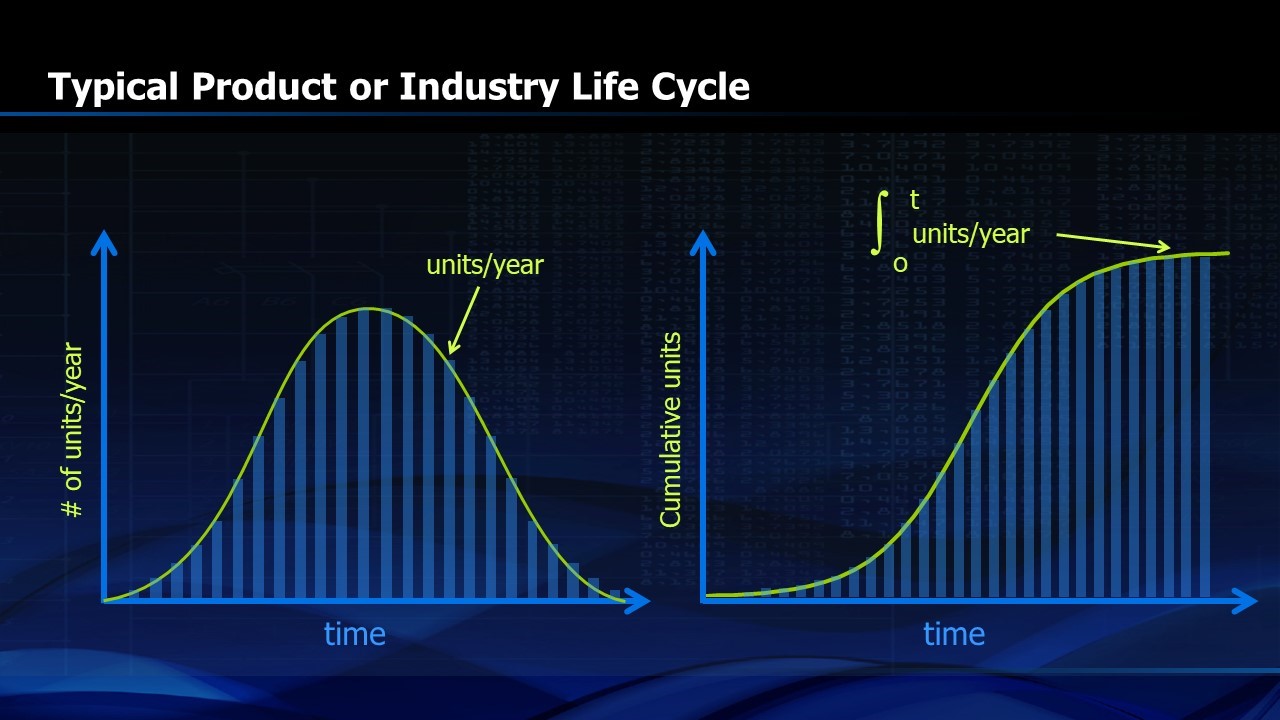
FIGURE 2. Typical product life cycle or life cycle of an industry
Figure 3 shows the stages of growth of the S-Curve. It starts out slow but the highest percentage growth is early in the S-Curve evolution. The curvature of the “S” increases upward until about 37% of the time on the horizontal axis is completed.2 Then the curvature is downward. Mathematically we would say that the second derivative of the Gompertz function is positive until about 37% of the time is completed and then the second derivative becomes zero. The rate of the rate of growth becomes negative and so the growth rate is less each year after that point.
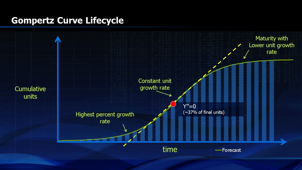
FIGURE 3. Gompertz Curve Life Cycle
I first became acquainted with the Gompertz Curve while managing a design project that TI was doing for IBM. IBM wanted us to report the number of simulated transistors that we had completed in our design each week. They then plotted them as a Gompertz Curve (Figure 4). Inexperienced project managers would have been frustrated by the fact that progress was initially very slow. The specification for the design project kept changing, new architectural approaches were tested and the number of simulated transistors remained small for some time. Then, things took off. The number of transistors completed each week grew linearly. Our inexperienced design manager would have been delighted and would have extrapolated this progress to an early completion as shown in Figure 4. With more experience, he would realize that the last fifth of the project would take more than one third of the total time.
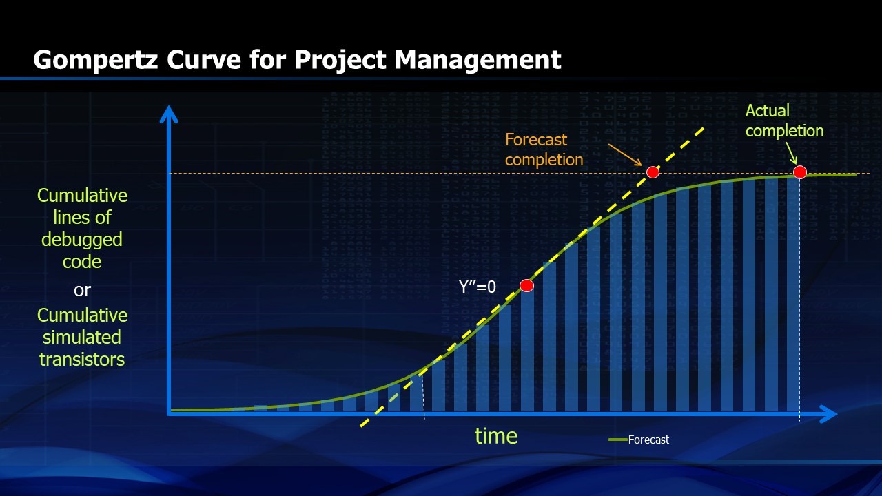
FIGURE 4. Use of Gompertz Curve for Project Management
While the Gompertz Curve is useful for project management, it provides even more insight for forecasting the future success of an embryonic product. Figure 5 shows the evolution of worldwide sales of notebook PCs. Using the data available to us with the actual shipments of PC notebooks in the years up through 2001, we can solve for the Gompertz coefficients a, b and c. We could then have used these coefficients to predict the future evolution of the growth curve for cumulative units of PC notebooks shipped. Figure 6 shows the Gompertz prediction versus the actual results reported in 2016. The results are nearly identical. If you were an aspiring competitor in the PC notebook business in 2001, or even an investor in the personal computer business, accurate knowledge of the future market for PC notebooks over the next fifteen years could be very useful.
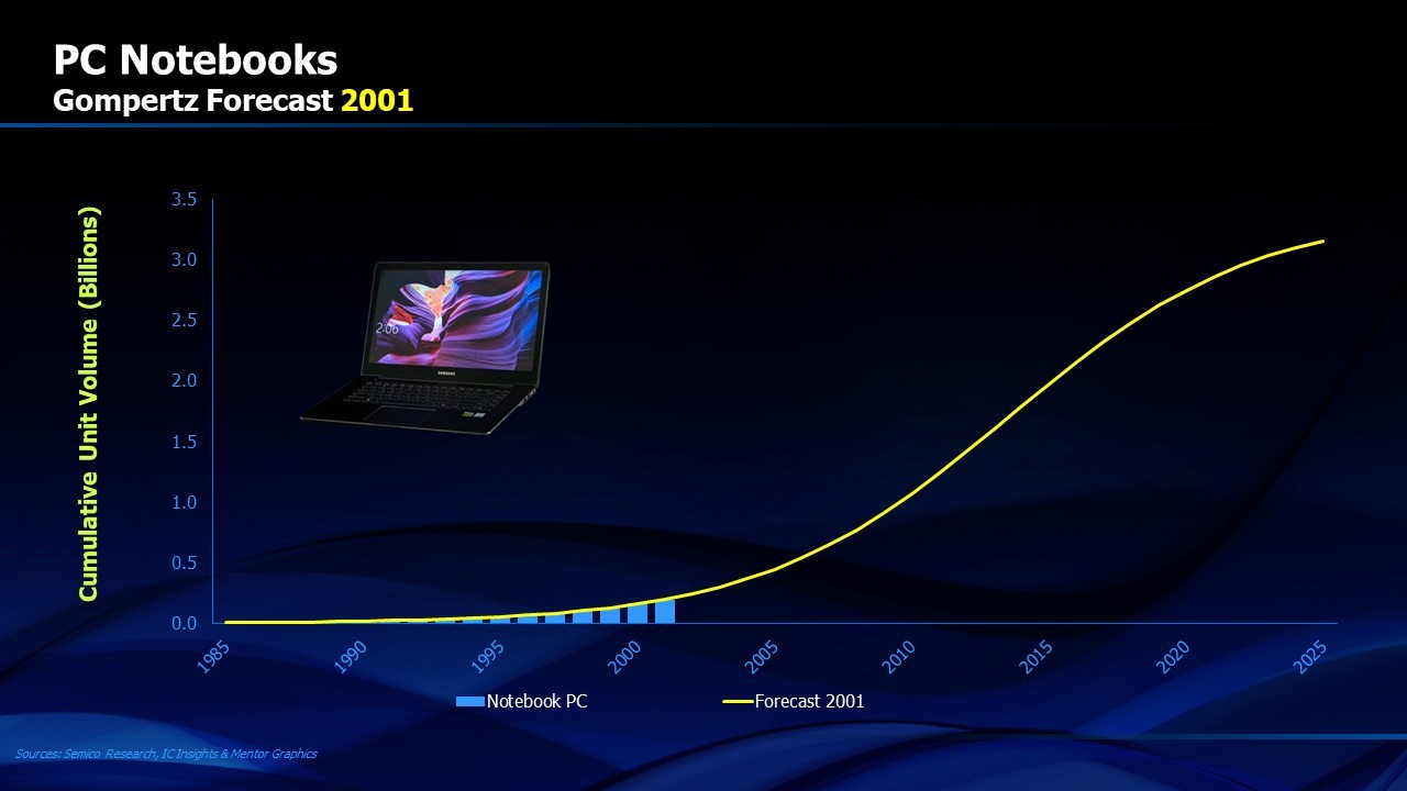
FIGURE 5. PC Notebook Shipments through 2001 provide data for Gompertz forecast
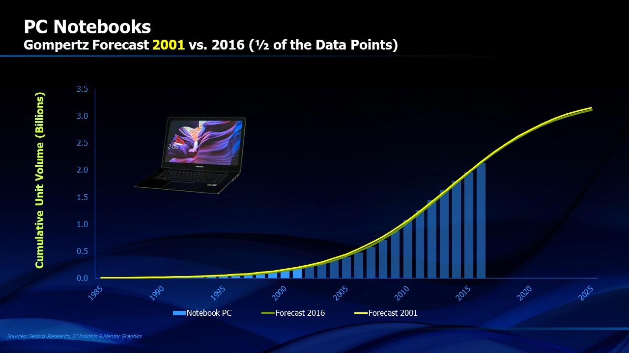
FIGURE 6. Actual PC Notebook shipments though 2016 (shown in green) versus Gompertz prediction in 2001 (shown in yellow)
Finally, Gompertz Curves can be used to predict the future of an industry. A good choice would be the future of the silicon transistor since lots of research dollars have been devoted to developing an alternative to the silicon switch and we don’t even know how soon we need it. Or do we? Gompertz analysis provides an opinion. It’s shown in Figure 7. Although the semiconductor industry and silicon technology may seem mature to some, we are in the infancy of our production of silicon transistors. The cumulative number of silicon transistors produced thus far is almost negligible compared to the future, as shown in Figure 7. The actual RATE of growth of shipments of silicon transistors is predicted to increase until about 2038. At that time, the Gompertz Curve suggests that the increase in the RATE of growth will become zero and the RATE of increase will be less each year until we reach saturation, sometime in the 2050 or 2060 timeframe. By then, we should have developed lots of alternatives.
![]()
Figure 7. Future of the silicon transistor
1https://en.wikipedia.org/wiki/Benjamin_Gompertz
2https://arxiv.org/ftp/arxiv/papers/1306/1306.3395.pdf
Share this post via:


Podcast EP357: How Gonka is Changing the Way AI is Accessed with David Liberman